Sensor Fusion
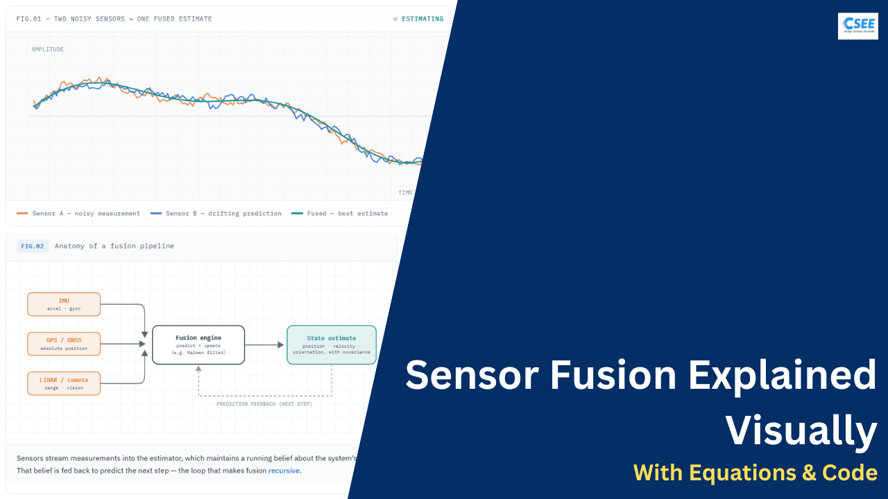
Every sensor lies a little. Sensor fusion is the craft of combining several imperfect measurements into one estimate that is more accurate, more reliable, and more complete than anything a single sensor could give you on its own.
Measurement
A raw reading from a sensor — e.g. an accelerometer or GPS fix. Often absolute, but noisy.
Prediction
What a model expects next — e.g. integrating a gyro or a motion model. Smooth, but it drifts.
Fused estimate
The corrected best guess after combining the two. Tighter uncertainty than either alone.
What is sensor fusion?
Sensor fusion is the process of merging data from two or more sensors so that the resulting information is better than what any single sensor could produce. “Better” can mean more accurate, less noisy, higher rate, more robust to failure, or simply possible — some quantities cannot be measured directly by any one device and only emerge when sources are combined.
A useful mental model is that fusion buys you three things at once:
- Complementarity — sensors with opposite weaknesses cover for each other. A gyroscope is smooth but drifts; an accelerometer is noisy but has a stable long-term reference. Together they are excellent.
- Redundancy — overlapping sensors increase confidence and let the system keep working when one drops out or is occluded.
- Coverage — combining modalities (range, vision, inertial) measures more of the world than any single modality can.
Almost every system that has to know where it is, how it’s oriented, or what’s around it relies on fusion: phones, drones, self-driving cars, VR headsets, spacecraft, and surgical robots all run a fusion engine at their core.
Sensors stream measurements into the estimator, which maintains a running belief about the system’s state. That belief is fed back to predict the next step — the loop that makes fusion recursive.
Why one sensor isn’t enough
No real sensor is perfect. Each one carries some mix of noise (random jitter), bias (a constant offset), drift (slowly accumulating error), limited range or field of view, a fixed update rate, and conditions where it simply fails. The trick is that these flaws are rarely shared — where one sensor is weak, another is usually strong.
Consider attitude (orientation) estimation, the classic case. A gyroscope reports rotation rate very smoothly and quickly, but integrating that rate to get an angle lets tiny errors pile up, so the estimate drifts. An accelerometer can sense the direction of gravity to give an absolute angle reference that never drifts — but it’s noisy and is fooled by any real acceleration. Each is useless alone for long; fused, they are rock-solid.
Notice how the blue and amber bars are almost mirror images. Fusion exploits exactly this: lean on each sensor only over the timescale where it is strong.
This is the whole intuition behind fusion in one picture. The job of a fusion algorithm is to weight each source according to how much it should be trusted right now — and to update those weights continuously as conditions change.
Levels of fusion
Fusion can happen at different stages of the processing chain. Engineers usually describe three levels, from raw signals up to final decisions. Which one you choose depends on bandwidth, compute budget, and how much you trust each raw stream.
Lower levels preserve the most information but demand precise alignment and calibration. Higher levels are robust and modular but discard detail. Many real systems mix levels.
- Data / raw-level — raw readings are combined directly (e.g. stacking LiDAR points and camera pixels into one representation). Maximum information, but requires tight spatial and temporal alignment.
- Feature-level — each stream is reduced to features first (corners, velocities, detected objects), and those features are merged. A good balance of richness and robustness.
- Decision-level — each sensor produces its own conclusion and the system combines the verdicts (voting, weighted averaging, Bayesian combination). Very robust and modular, but the most information is lost.
The probabilistic foundation
Modern fusion is built on probability. Instead of treating a measurement as a single exact number, we treat it as a belief: a most-likely value plus an honest statement of how uncertain we are. For many problems that belief is modeled as a Gaussian — a bell curve described by a mean (μ, the estimate) and a variance (σ², the spread). More uncertainty means a wider, flatter curve.
The beautiful result is this: when you multiply two Gaussian beliefs together, you get another Gaussian — and it is narrower than either input. Combining information can only reduce uncertainty. This single fact is the engine inside the Kalman filter.
The amber and blue beliefs each have wide spread. Their product (teal) sits between them, leans toward the more confident one, and is taller and narrower — lower uncertainty than either source.
For real systems the state is usually a vector (position and velocity and orientation), so the variance becomes a covariance matrix that also captures how variables relate. The picture generalizes from a bell curve to an ellipse: a tight ellipse means a confident estimate, a fat one means we’re unsure.
The complementary filter
The gentlest entry point to fusion is the complementary filter. It needs no probability theory and runs in a handful of lines, which is why it’s everywhere in drones and hobby IMUs. The idea: pass each sensor through the frequency band it’s good at, then add the results.
For tilt estimation, the gyroscope is trustworthy over short times (high frequencies) and the accelerometer over long times (low frequencies). So we high-pass the integrated gyro and low-pass the accelerometer angle, and blend them with a single weight α (typically 0.95–0.99):
The gyro carries the fast motion; the accelerometer quietly pulls the estimate back toward true vertical so drift never accumulates. One tunable knob, α, sets the crossover.
The complementary filter is a fixed-gain special case of what comes next. Its weakness is that α is constant — it can’t adapt when a sensor temporarily becomes unreliable. To make the weighting respond to live uncertainty, we need the Kalman filter.
The Kalman filter
The Kalman filter is the workhorse of sensor fusion. It maintains a Gaussian belief about the state and updates it in an endless two-step rhythm: predict where things should be using a motion model, then update that prediction with each new measurement. Crucially, it tracks not just the estimate but its covariance, so it always knows how much to trust itself.
Predict uses physics to guess the next state and widens uncertainty; update folds in a measurement and tightens it. The output of one cycle is the input to the next.
The single most important quantity is the Kalman gain K. It is the filter’s live trust dial, computed every step from the relative uncertainties of the prediction (P) and the measurement (R):
- When the measurement is precise (small R), K is large → the filter leans on the measurement.
- When the measurement is noisy (large R), K is small → the filter trusts its own prediction instead.
This is exactly the complementary filter’s blend, except the weight is recomputed continuously and optimally from the data. The two tuning matrices you choose are Q (how much you trust your motion model) and R (how noisy each sensor is). Get these right and the filter is remarkably good; get them wrong and it either ignores reality or chases noise.
EKF, UKF & particle filters
The plain Kalman filter assumes the world is linear. Reality — rotations, range measurements, camera projection — rarely is. Three families of estimator handle nonlinearity, trading accuracy against compute.
- Extended Kalman Filter (EKF) — linearizes the nonlinear model at the current estimate using its derivatives (Jacobians), then runs the ordinary Kalman equations. Cheap and ubiquitous, but the approximation can break down when nonlinearity is strong.
- Unscented Kalman Filter (UKF) — instead of linearizing, it samples a small, carefully chosen set of sigma points, pushes each through the true nonlinear function, and reconstructs the resulting mean and covariance. More accurate than the EKF, no derivatives required, only modestly more expensive.
- Particle filter — represents the belief with hundreds or thousands of weighted samples, so it can handle arbitrary, multi-peaked, non-Gaussian distributions. The most general and the most computationally hungry; common in robot localization (e.g. Monte Carlo localization).
The EKF forces a straight-line fit through a curve; the UKF lets representative points flow through the real nonlinearity and measures what comes out. When the function bends sharply, the UKF’s estimate stays truer.
A practical rule of thumb: start with an EKF, move to a UKF if accuracy suffers and derivatives are painful, and reach for a particle filter only when the belief genuinely can’t be captured by a single bell curve — for instance, “I’m in one of three identical corridors.”
Worked example: IMU + GPS
The canonical fusion problem ties everything together: estimating a vehicle’s pose by combining a fast, drifting IMU with a slow, absolute GPS. The IMU updates hundreds of times a second but accumulates drift; GPS arrives only a few times a second but never drifts. Fused, you get a smooth, high-rate, drift-free trajectory.
The filter runs the predict step on every IMU sample — dead-reckoning the pose forward — and runs the update step only when a GPS fix arrives, snapping the accumulated drift back to the absolute reference.
Between GPS fixes the error climbs as the IMU dead-reckons; each amber correction pulls it back down. The teal estimate stays tightly bounded — smooth like the IMU, anchored like GPS.
This same skeleton — fast predictor plus slower absolute corrector — appears in visual-inertial odometry (camera + IMU), wheel-encoder + LiDAR localization, and underwater navigation. Once you see the pattern, you see it everywhere.
Frames, calibration & timing
The filter math gets the attention, but in practice three unglamorous details decide whether fusion works at all: coordinate frames, calibration, and time synchronization. Get any of them wrong and a perfect filter will confidently produce garbage.
Every sensor measures in its own reference frame. A camera sees in its optical frame, an IMU in the body frame, GPS in a world frame. Before anything can be fused, all measurements must be expressed in one common frame, using a known rotation R and translation t between them.
Finding R and t between sensors is extrinsic calibration; correcting each sensor’s internal model (lens distortion, gyro bias) is intrinsic calibration. Both must be done before fusion is meaningful.
- Calibration — extrinsic (where sensors sit relative to each other) and intrinsic (each sensor’s internal parameters). Small errors here masquerade as motion and corrupt the estimate.
- Time synchronization — measurements must carry accurate timestamps on a shared clock. If a 200 Hz IMU sample is matched to the wrong GPS time, the filter fuses inconsistent data. Hardware-triggered timestamps beat software ones.
- Outlier rejection — a single bad reading (a GPS multipath spike) can yank the estimate. Filters gate measurements by how surprising they are (the innovation) and discard the implausible ones.
Where it’s used
Sensor fusion is invisible infrastructure — once you know the shape of it, you’ll spot it in nearly every device that perceives the physical world.
Autonomous vehicles
LiDAR, radar, cameras, IMU and GPS fuse into one model of the road and the car’s place on it.
Drones
IMU + barometer + GPS + optical flow keep a quadcopter stable and aware of its position mid-air.
AR / VR headsets
Inertial + camera tracking fuse to place virtual objects steadily in the real room.
Phones & wearables
Step counting, orientation, and indoor navigation come from fusing tiny MEMS sensors.
Robotics
Wheel odometry, LiDAR and depth cameras fuse for mapping and reliable localization (SLAM).
Aerospace
Star trackers, IMUs and GNSS fuse to navigate aircraft, satellites and spacecraft.
Practical tips & pitfalls
A few hard-won lessons separate a fusion system that works in the lab from one that works in the world:
- Tune Q and R deliberately. R should reflect each sensor’s real noise (check the datasheet, then verify empirically). Q encodes how much you trust your motion model. These two matrices are where most of the engineering time goes.
- Garbage in, garbage out. The cleverest filter cannot rescue uncalibrated sensors, wrong frames, or bad timestamps. Fix the data path first.
- Gate your measurements. Reject readings whose innovation is wildly larger than expected — they’re almost always faults, not surprises worth believing.
- Watch observability. Some states simply can’t be recovered from your sensor set (e.g. absolute heading from accel + gyro alone). Know what your sensors can and cannot reveal before trusting the output.
- Start simple. A complementary filter or basic Kalman filter often does the job. Add EKF/UKF/particle complexity only when measurements prove you need it.
- Sanity-check the covariance. If the filter’s reported uncertainty stops matching reality, it has become overconfident — a classic, dangerous failure mode.
Build it: a Kalman filter in code
Time to put every piece together into something you can actually run. The scenario: a vehicle drives down a straight road at a steady speed. A GPS-like sensor reports its position ten times a second, but each reading is off by about two metres — and it never measures speed. The goal is a smooth position estimate and a recovered velocity, using a constant-velocity Kalman filter: the simplest filter that still exercises the full predict–update machinery.
-
Define the state and motion model
Track position and velocity together. A constant-velocity model says next position = position + velocity·Δt, and velocity stays put. We only observe position, so the measurement matrix H picks it out.
modelx = [ p , v ]ᵀ // state: position, velocityF = [[ 1 , Δt ], [ 0 , 1 ]] // constant-velocity transitionH = [ 1 , 0 ] // we measure position only -
Choose the noise
Q models the motion we left out — random acceleration with standard deviation σa. R is the sensor’s measurement variance σz². These two knobs decide how much the filter trusts its model versus its sensor.
noiseQ = σa² · [[ Δt⁴/4 , Δt³/2 ], [ Δt³/2 , Δt² ]] // unmodeled accelR = [ σz² ] // sensor noise variance -
Predict
Project the state forward with the model, and grow the uncertainty by Q because the model is imperfect.
predictx̂⁻ = F · x̂P⁻ = F · P · Fᵀ + Q -
Update with the measurement
Compare the prediction to the reading (the innovation y), compute how much to trust the reading (the gain K), then correct both the state and the covariance.
updatey = z − H · x̂⁻ // innovation (the surprise)S = H · P⁻ · Hᵀ + R // innovation covarianceK = P⁻ · Hᵀ · S⁻¹ // Kalman gainx̂ = x̂⁻ + K · y // corrected stateP = ( I − K · H ) · P⁻ // corrected covariance
To make it concrete, here is the very first cycle worked out with the actual first measurement, z₁ = 0.351 m. Starting from a position/velocity uncertainty of 10 and a sensor variance of R = σz² = 4:
Notice what one cycle did: the position variance collapsed from 10.1 to 2.87 because the measurement was informative, while the velocity variance barely moved. We never measure velocity directly — the filter can only infer it, tightening it over many cycles as position estimates accumulate. That inference is the whole magic.
Here is the complete filter. It needs only NumPy; the synthetic truth and noisy readings stand in for a real sensor log.
import numpy as np

# 1. MODEL — constant-velocity: state x = [position, velocity]
dt = 0.1                                   # time step (s)
F  = np.array([[1, dt],                    # state transition
               [0,  1]])
H  = np.array([[1, 0]])                    # measure position only

sigma_a = 0.2                              # process-noise accel std (m/s^2)
Q = sigma_a**2 * np.array([[dt**4/4, dt**3/2],
                           [dt**3/2, dt**2 ]])
sigma_z = 2.0                              # measurement-noise std (m)
R = np.array([[sigma_z**2]])

# 2. INITIAL BELIEF
x = np.array([[0.0], [0.0]])               # guess: at origin, at rest
P = np.eye(2) * 10.0                       # but very unsure (large P)

# 3. SYNTHETIC TRUTH + NOISY GPS-LIKE MEASUREMENTS
rng    = np.random.default_rng(0)
N      = 100
true_p = np.cumsum(np.full(N, 1.0 * dt))   # vehicle moves at 1 m/s
meas   = true_p + rng.normal(0, sigma_z, N)

# 4. RUN THE FILTER
I   = np.eye(2)
est = []
for z in meas:
    # predict
    x = F @ x
    P = F @ P @ F.T + Q
    # update
    z = np.array([[z]])
    y = z - H @ x                   # innovation (the surprise)
    S = H @ P @ H.T + R             # innovation covariance
    K = P @ H.T @ np.linalg.inv(S)  # Kalman gain
    x = x + K @ y                   # corrected state
    P = (I - K @ H) @ P             # corrected covariance
    est.append((x[0, 0], x[1, 0]))

p, v = est[-1]
print(f"position: {p:.2f} m   (true {true_p[-1]:.2f})")
print(f"velocity: {v:.2f} m/s  (true 1.00, never measured directly)")
position: 10.20 m   (true 10.00)
velocity: 0.98 m/s  (true 1.00, never measured directly)
Amber dots are the raw ~2 m-noise readings; the teal line is the filter’s estimate tracking the dashed true path. Over the run, position error drops from 1.93 m (raw) to 0.76 m (filtered).
Thirty lines, and the filter recovers a velocity it was never given (0.98 m/s vs. a true 1.00) and roughly halves the position error. Swap in your sensor’s real noise figures, extend the state to two dimensions or add orientation, and this exact skeleton — predict, then correct — scales straight up to the IMU + GPS systems from earlier.