Hardware-in-the-Loop Testing with dSPACE
A complete, diagram-driven walkthrough of how a real Electronic Control Unit is tested against a simulated world running in real time — the architecture, the boxes, the wiring, the solvers, the bus simulation, the fault injection, and the automation that ties it together.
What Hardware-in-the-Loop Actually Is
Hardware-in-the-Loop (HiL) testing is a technique for validating an embedded controller by connecting the real physical controller to a computer that simulates the rest of the world in real time. The controller believes it is installed in a finished vehicle, aircraft, wind turbine, or power converter. In reality, every sensor it reads and every actuator it commands is being emulated by a real-time simulator so faithfully that the controller cannot tell the difference. That simulator, in the automotive and aerospace industries, is very often built from dSPACE hardware and software.
The core idea is a closed loop. The Electronic Control Unit (ECU) — the “Device Under Test” or DUT — sends actuator commands. The real-time simulator receives those commands through its output channels, feeds them into a mathematical model of the plant (the engine, the brakes, the battery, the motor), computes how the plant responds, and drives sensor-emulation signals back into the ECU’s inputs. The ECU reacts to those sensor readings, issues new commands, and the loop closes again — typically hundreds or thousands of times per second. Because the plant is software, you can test conditions that would be dangerous, expensive, or physically impossible to reproduce on a real prototype: a wheel locking on black ice, a battery cell going into thermal runaway, a sensor wire breaking at 200 km/h, a lambda probe drifting out of calibration.
The word that makes HiL hard is real time. A desktop simulation can pause, slow down, or take as long as it needs to compute a millisecond of plant behaviour. A HiL simulator cannot. It is wired to a physical controller that runs on its own clock and expects fresh, physically correct sensor signals at deterministic intervals. If the simulator computes one step of the plant model in less time than the real-world interval it represents, the loop stays honest. If it ever takes longer — an overrun — the illusion breaks and the test is invalid. Everything about a dSPACE HiL system, from the processor boards to the solver choice to the way I/O is scheduled, exists to guarantee that this real-time deadline is never missed.
Why teams invest in HiL
- Safety. You can inject faults and drive the plant into destructive regimes without endangering people or equipment.
- Coverage. Rare corner cases, sensor failures, and extreme environmental conditions can be reproduced on demand and exactly repeated.
- Repeatability. A simulated plant behaves identically every run, which is essential for regression testing and for chasing intermittent bugs.
- Automation. Thousands of test cases can run overnight, unattended, with automatic pass/fail evaluation and reporting.
- Cost and time. Testing starts long before a physical prototype exists, and one HiL bench replaces many test drives.
- Parallelisation. Multiple ECUs and multiple test teams can work against identical benches simultaneously.
In HiL, the controller is real hardware and the plant is simulated. This is the mirror image of Rapid Control Prototyping (RCP), where the controller is simulated on fast hardware and the plant is real. Knowing which half of the loop is real is the fastest way to identify any test setup you encounter.
How this tutorial is organised
The sections below move from concept to concrete. We place HiL inside the V-model of embedded development, build up the physical architecture of a dSPACE bench, tour the real hardware boxes and the I/O that connects them to the ECU, walk through the full software toolchain, and then get into the parts engineers find hardest: the plant model, the real-time solver algorithms, bus and restbus simulation, electrical fault injection, timing and task scheduling, and finally test automation. Every major concept is paired with a scalable diagram and, where a comparison helps, a table.
HiL in the V-Model and the Ladder of Test Levels
Embedded control software is almost universally developed against the V-model. The left-hand descending arm of the V captures requirements and design, moving from system requirements down through software architecture to detailed component design and code. The right-hand ascending arm captures integration and verification, moving from unit tests back up to full system acceptance. Each level on the right verifies a corresponding level on the left. HiL lives near the top of the right arm: it is the last major verification stage before a controller is validated in a real vehicle.
It helps to see HiL as the top rung of a ladder of “in-the-loop” methods, each of which keeps more of the system real. As you climb the ladder, fidelity and confidence rise, but so do cost, complexity, and execution time.
| Level | Controller | Plant | Runs on | Real-time? | Primary purpose |
|---|---|---|---|---|---|
| MiL Model-in-the-Loop | Model (Simulink) | Model (Simulink) | Engineering PC | No | Verify control algorithm logic against a plant model, early in design. |
| SiL Software-in-the-Loop | Generated C code | Model | Engineering PC (e.g. VEOS) | No | Confirm the generated production code behaves like the model. |
| PiL Processor-in-the-Loop | Code on target CPU / eval board | Model | Target processor + host | Partial | Check code on the real instruction set: timing, fixed-point, compiler effects. |
| HiL Hardware-in-the-Loop | Real ECU hardware | Model on RT simulator | dSPACE real-time system | Yes | Validate the finished controller with real I/O, buses, and electrical behaviour. |
A well-run program uses all four. MiL catches algorithmic mistakes when they are cheapest to fix. SiL guarantees the auto-generated code is faithful to the model. PiL exposes processor-specific effects such as fixed-point overflow or timing jitter. Only HiL, however, exercises the actual pins of the actual ECU: its analog-to-digital converters, its output drivers, its transceivers, its watchdog, its power supply behaviour, and its diagnostic reactions to genuine electrical faults. That is why HiL is indispensable for safety-relevant systems governed by standards such as ISO 26262 in automotive or DO–178C in aerospace, where evidence of thorough, repeatable verification is mandatory.
dSPACE provides tools across this whole ladder — VEOS for SiL, MicroLabBox and SCALEXIO for HiL — but the company’s flagship strength, and the focus of this tutorial, is real-time HiL on SCALEXIO hardware driven by ConfigurationDesk, ControlDesk, and AutomationDesk.
The Closed Real-Time Loop
Every HiL bench, no matter how large, is built from the same five architectural blocks arranged in a loop. Understanding this loop is the single most useful mental model in the entire discipline, because every piece of hardware and every software tool exists to serve one of these blocks.
- The ECU (Device Under Test). The real controller, powered and wired exactly as it would be in the target system.
- The I/O interface. The hardware that converts between the ECU’s electrical pins and the simulator’s digital numbers — digital-to-analog and analog-to-digital converters, digital lines, PWM capture and generation, and bus transceivers.
- The real-time processor. The computing engine that runs the plant model at a fixed step, in lockstep with wall-clock time.
- The plant model. The mathematical description of the physical world — engine, driveline, battery, motor, hydraulics — that turns actuator commands into sensor values.
- Signal conditioning and loads. The amplifiers, level shifters, electronic loads, and failure-insertion units that make emulated signals electrically realistic and let you break them on command.
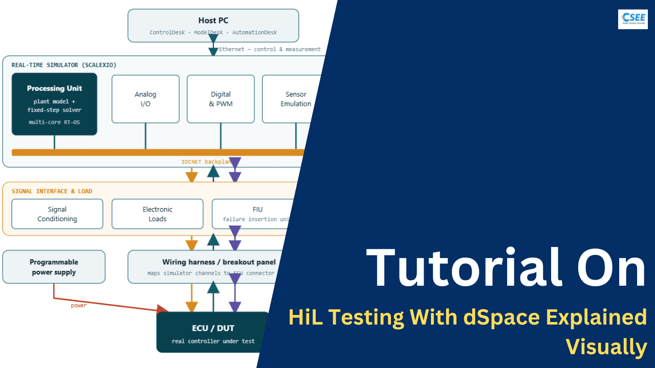
The closed loop above is the concept. In practice it is realised by a stack of physical components arranged in layers. The architecture diagram below shows a complete bench with all of its main building blocks: the host PC, the real-time simulator and its I/O boards, the signal-interface layer that makes the electrical connection honest, the wiring harness, the programmable power supply, and the ECU under test.
Following one loop iteration
Trace a single control cycle to see how the blocks cooperate. Suppose the ECU is an engine controller and the loop runs at 1 kHz (a 1 ms step):
- Read. At the start of the step, the I/O hardware samples every ECU output the model needs: injector pulse widths, ignition timing, throttle command, fuel-pump PWM duty. Analog outputs pass through ADCs; digital and PWM outputs are timed by capture units.
- Compute. Those numbers become inputs to the plant model. The real-time solver advances the engine, air-path, and driveline equations by exactly one 1 ms step, producing new physical states: crank angle, manifold pressure, engine speed, exhaust lambda.
- Write. The model’s outputs are converted back to electrical signals. Crank and cam positions become emulated Hall or VR sensor waveforms; manifold pressure becomes an analog voltage; lambda becomes a conditioned probe signal. DACs, digital pattern generators, and dedicated sensor-emulation channels drive the ECU’s input pins.
- React. The ECU reads those emulated sensors, runs its own control law, and issues fresh actuator commands — which the I/O will capture at the start of the next step.
All of this must finish inside the 1 ms budget, every single millisecond, for as long as the test runs. The host PC, meanwhile, sits alongside the loop: it lets an engineer watch signals, change parameters, calibrate the model, log data, and run automated test sequences — but it is deliberately kept out of the real-time path so that a slow disk write or a busy operating system can never cause the loop to miss its deadline.
A HiL simulator is not merely “a fast PC.” Its defining property is determinism: the same step always takes a bounded, predictable amount of time. A general-purpose operating system cannot promise that. This is why dSPACE real-time hardware runs a dedicated real-time environment on isolated processor cores, with I/O handled by FPGAs and dedicated boards rather than by interrupt-driven drivers on a shared CPU.
The dSPACE Hardware Family
dSPACE real-time systems come in several form factors that trade portability against channel count and scalability. Choosing the right one is the first hardware decision in any project.
SCALEXIO — the modern HiL workhorse
SCALEXIO is dSPACE’s scalable HiL platform and the backbone of most serious benches built today. Its philosophy is modularity: a SCALEXIO system is assembled from a processing unit plus a set of I/O boards, each occupying a slot in a rack, connected over a high-speed internal bus called IOCNET. Because IOCNET can span multiple racks, a SCALEXIO system scales from a compact single-ECU tester up to a full networked bench emulating an entire vehicle with dozens of ECUs.
The processing hardware uses standard multi-core Intel processors running a dSPACE real-time operating system. This matters: because the CPU is a mainstream x86 part, plant models with heavy computational load — detailed electric-motor models, multi-cylinder combustion, high-order battery models — run comfortably, and you can distribute a large model across multiple cores. The I/O boards are where the real specialisation lives; each board is a focused instrument for a class of signals, often with its own FPGA for microsecond-accurate timing independent of the CPU.
MicroLabBox — the compact all-rounder
MicroLabBox is a benchtop unit that combines a real-time processor and a rich, fixed set of I/O in one small chassis. It is popular in universities and R&D labs for small HiL setups and rapid control prototyping because it is affordable, easy to wire, and needs no rack. Its I/O count is fixed rather than expandable, so it suits single-ECU or component-level testing rather than full-vehicle benches.
MicroAutoBox — in-vehicle prototyping
MicroAutoBox is a rugged, compact real-time computer designed to be installed in a moving vehicle. Strictly it is a prototyping controller (RCP) rather than a HiL simulator, but it appears constantly in the same workflows: engineers use it to run a prototype control algorithm in a real car before the production ECU exists, and the same models later run against a SCALEXIO HiL bench. It tolerates automotive temperature, vibration, and power conditions that a lab box never sees.
| Platform | Role | Form factor | I/O model | Scales to full vehicle? | Typical use |
|---|---|---|---|---|---|
| SCALEXIO | HiL simulator | Rack / modular | Expandable boards | Yes | Production HiL, multi-ECU network benches |
| MicroLabBox | HiL & RCP | Benchtop | Fixed, integrated | Limited | Labs, teaching, component HiL, prototyping |
| MicroAutoBox | RCP (in-vehicle) | Rugged compact | Fixed, automotive | No | Prototype controllers in real vehicles |
| VEOS | SiL (virtual) | Software only | Virtual | Virtual | PC-based SiL before hardware exists |
What the I/O boards actually do
Inside a SCALEXIO rack, boards fall into recognisable families. Analog boards generate precise voltages and currents to emulate sensors, and measure the ECU’s analog outputs. Digital and PWM boards capture the ECU’s pulse-width-modulated actuator commands (injectors, valves, motor phases) with sub-microsecond timing, and generate digital patterns back to the ECU. Bus boards host CAN, CAN FD, LIN, FlexRay, and Automotive Ethernet transceivers for network communication and restbus simulation. Sensor-emulation boards synthesise specialised waveforms such as crankshaft/camshaft signals, resolver and encoder signals for electric motors, and wheel-speed patterns. Electronic load and failure-insertion boards present realistic loads to the ECU’s output drivers and can electrically break, short, or corrupt any channel on command. We return to the last two in the sections on I/O and fault injection.
Count the ECU’s connector pins by function first — how many analog inputs, how many PWM outputs, how many bus nodes, how many sensor waveforms — and only then pick boards. Under-provisioning I/O is the most common and most painful HiL planning mistake, because adding a board later can mean rewiring the whole loom.
Signal Types, Conditioning, and the Electrical Interface
The I/O layer is where the abstract world of the model meets the stubborn reality of electronics. An ECU does not read floating-point numbers; it reads voltages, currents, frequencies, edges, and bus frames, and it is exquisitely sensitive to their electrical quality. The job of the I/O and signal-conditioning layer is to make emulated signals so electrically convincing that the ECU’s input circuitry — its dividers, filters, comparators, and ADCs — responds exactly as it would to a real sensor.
The main signal classes
| Signal class | Examples | Direction | dSPACE handling |
|---|---|---|---|
| Analog voltage | MAP, TPS, temperature, potentiometers | Sim → ECU | DAC + conditioning to match source impedance & range |
| Analog measurement | ECU driver output voltage/current | ECU → Sim | ADC with appropriate range & isolation |
| Resistive | NTC/PTC temperature, position sensors | Sim → ECU | Programmable resistor / current-based emulation |
| Digital / switch | Ignition, door, brake switches | Both | Digital I/O, level-shifted to ECU domain |
| PWM (out) | Injector, valve, pump, fan commands | ECU → Sim | FPGA capture of duty & frequency, sub-µs |
| PWM (in) | Sensor duty-cycle signals | Sim → ECU | FPGA-timed pattern generation |
| Crank / cam | Engine position (VR / Hall) | Sim → ECU | Dedicated angle-based sensor-emulation channel |
| Resolver / encoder | e-motor rotor position | Sim → ECU | Resolver/encoder emulation board |
| Bus frames | CAN, LIN, FlexRay, Ethernet | Both | Transceivers + protocol engine (restbus) |
| Power / high-current | Actuator loads, relays | ECU → load | Electronic loads emulating real actuator impedance |
Why raw DAC output is not enough: signal conditioning
A digital-to-analog converter can produce a clean 0–5 V signal, but the ECU expects that signal to come from a specific kind of source. A real temperature sensor is a resistor in a divider; a real pressure sensor has a defined output impedance and drive capability; a real wheel-speed sensor produces a particular current waveform. Signal conditioning is the analog electronics between the DAC and the ECU pin that reshapes an ideal signal into a realistic one: adjusting output impedance, level, drive current, and filtering so the ECU’s front end cannot distinguish emulation from reality. Get this wrong and the ECU may still “work,” but it will read subtly wrong values or flag a plausibility fault — and you will chase a phantom software bug that is really an impedance mismatch on the bench.
Electronic loads: giving the ECU something to push against
An ECU output driver expects to drive a real load — the coil of an injector, the winding of a solenoid, the filament of a lamp. If you leave that pin open, the driver’s current-sense and diagnostic circuitry sees “open load” and flags a fault; if you short it to a fixed resistor, the transient behaviour is wrong. Electronic loads emulate the correct impedance, including inductive and dynamic behaviour, so that the ECU’s driver diagnostics are satisfied and the measured current waveform is realistic. For inductive actuators, the load must reproduce the flyback and current-decay characteristics the ECU’s driver expects, which is why dedicated load boards, rather than plain resistors, are used.
A huge fraction of first-power-on HiL problems are grounding problems. The simulator, the ECU power supply, and the signal conditioning must share a clean, well-defined reference. Ground loops introduce noise that shows up as jittery analog reads or spurious diagnostic trouble codes. Plan the grounding scheme as deliberately as the signal wiring.
The dSPACE Software Toolchain
Hardware is only half of a HiL system. The dSPACE software toolchain takes a plant model built in MATLAB/Simulink, maps its inputs and outputs onto real I/O channels, generates real-time code, downloads it to the processor, and gives engineers a live cockpit to run and automate tests. Each tool owns one stage of that pipeline.
| Tool | Stage | What it does |
|---|---|---|
| RTI / RTI-MP | Model → hardware | Real-Time Interface: Simulink blockset that connects model signals to dSPACE I/O; MP variant handles multiprocessor/multi-core. |
| ConfigurationDesk | I/O mapping & build | Graphically maps model ports to physical channels, configures signal properties, generates and builds the real-time application for SCALEXIO. |
| Model / Simulink + TargetLink | Plant & controller code | Plant model authoring; TargetLink generates production-grade controller C code for SiL/PiL. |
| ControlDesk | Experiment / runtime | The operator cockpit: instrument panels, live parameter tuning, measurement, data logging, calibration access (XCP/CCP). |
| ModelDesk | Parameterisation | Manages road, maneuver, and vehicle-model parameters; drives scenario definition for vehicle-dynamics models (ASM). |
| MotionDesk | Visualisation | 3-D animation of the simulated vehicle/scene for driver-in-the-loop and ADAS work. |
| AutomationDesk | Test automation | Builds, runs, and documents automated test sequences; scriptable in Python for regression suites. |
| ASM | Plant model library | Automotive Simulation Models: ready-made, validated Simulink plant models (engine, vehicle dynamics, e-motor, battery, traffic). |
| VEOS | Virtual validation | PC-based simulation platform for SiL, letting the same models run without HiL hardware. |
| SystemDesk | AUTOSAR architecture | Authors AUTOSAR software architectures and generates virtual ECUs (V-ECUs) for SiL. |
| RTMaps | Sensor data flow | Time-stamped multi-sensor data handling, heavily used in ADAS/autonomous HiL. |
RTI and ConfigurationDesk: the crucial mapping step
A plant model has abstract ports named things like engine_speed or injector_duty. Those names mean nothing to a piece of copper. ConfigurationDesk is where an engineer draws the correspondence: this model output goes to that DAC channel on that board with this scaling; this PWM-capture channel feeds that model input. It also defines electrical properties — ranges, pull-ups, termination — and, critically, it generates and compiles the real-time application that will run on the SCALEXIO processor. On older PHS-bus systems, the equivalent job was done with the RTI blockset directly inside Simulink; ConfigurationDesk is the modern, board-aware successor for SCALEXIO.
ControlDesk: the operator’s cockpit
Once the application runs, ControlDesk is the window into it. Engineers build layouts full of virtual instruments — gauges, plotters, numeric displays, sliders, switches — each bound to a model variable. You can watch a signal in real time, change a parameter live to see how the ECU reacts, record measurements to disk for later analysis, and access the ECU’s own internal variables through calibration protocols such as XCP and CCP. ControlDesk is also where measurement data is captured for automated pass/fail evaluation.
Building a validated engine or full-vehicle plant model from scratch is a multi-year effort. dSPACE’s ASM library ships ready-made, physically validated Simulink models for combustion engines, vehicle dynamics, electric drives, batteries, and even traffic and sensors for ADAS. Most teams start from ASM and customise, rather than modelling the plant from first principles.
The Plant Model: Physics That Closes the Loop
The plant model is the intellectual heart of a HiL system. It is a set of mathematical equations that, given the ECU’s actuator commands and the current physical state, computes how the physical world evolves and what the sensors would read. Its fidelity determines how meaningful your test results are: a model that is too crude will let bugs slip through, while a model that is too detailed may be impossible to run in real time.
State-space thinking
Most plant models are, at bottom, systems of ordinary differential equations (ODEs) written in state-space form. The plant has a vector of states x (positions, velocities, temperatures, pressures, charges), receives a vector of inputs u (the ECU’s actuator commands plus any environmental drivers), and produces a vector of outputs y (the sensor readings). The dynamics are:
Ẋ is a function of the current state and inputs; the sensor outputs are an algebraic function of state and inputs. The solver’s job is to integrate the first equation forward in time.For example, a simplified vehicle longitudinal model might have states of position and velocity, an input of drive torque (commanded by the ECU) and road grade (an environmental input), and outputs of wheel speed and accelerometer reading (the sensors the ECU reads). The equation Ẋ = f(x,u) encodes Newton’s second law plus rolling resistance and aerodynamic drag; the output equation y = g(x,u) converts states into what each sensor would measure.
Model fidelity is a spectrum
The same physical system can be modelled at many levels of detail, and the right choice depends on what the ECU is being tested for.
- Functional / mean-value models capture average behaviour cheaply. A mean-value engine model tracks air mass, fuel, and torque without resolving individual combustion events. It runs fast and is ideal for testing higher-level control and diagnostics.
- Crank-angle-resolved models resolve each combustion event as a function of crankshaft angle. They are essential when testing cylinder-individual control, misfire detection, or knock control, but they demand small step sizes and more computation.
- High-fidelity physical models (detailed multibody dynamics, distributed thermal networks, electrochemical battery models) give the most realism but can be too heavy for real time and are often reserved for offline analysis.
| Test goal | Model type | Typical step | Real-time cost |
|---|---|---|---|
| Diagnostics, comms, supervisory logic | Mean-value / functional | 1 ms | Low |
| Torque & emissions control | Crank-angle engine | 0.1–1 ms | Medium |
| Inverter / e-motor control | Switched power electronics | 1–10 µs (FPGA) | High |
| Vehicle dynamics / ADAS | Multibody + tyre + sensors | 1 ms | Medium |
| Battery management | Equivalent-circuit / electro-thermal | 1–10 ms | Low–Med |
The FPGA tier for very fast dynamics
Some dynamics are simply too fast for a CPU running at a 1 ms step. Power-electronic inverters switch at tens of kilohertz, so their current ripple lives on a microsecond timescale. To emulate a motor and inverter faithfully, that fast electrical model must run on an FPGA at microsecond or sub-microsecond steps, while the slower mechanical and thermal parts of the model run on the CPU at 1 ms. dSPACE supports exactly this split: an FPGA I/O board runs the fast switching model, and the CPU runs the rest, exchanging data each CPU step. This multi-rate, multi-processor partitioning is one of the defining skills of advanced HiL engineering.
There is no universally “correct” plant model — only a model appropriate to the test. Always ask: what must the ECU see for this test to be valid? Model exactly that, at the coarsest fidelity that still fools the ECU, and no finer. Excess fidelity costs step time you cannot spare.
Solver Algorithms and Real-Time Integration
The plant model gives you Ẋ = f(x,u). A solver turns that derivative into an actual trajectory by integrating it forward in time. On a desktop you can use a clever variable-step solver that shrinks the step when things get tricky and grows it when they are smooth. On a HiL bench you cannot: the loop must advance by a fixed amount every fixed interval, forever. This single constraint — fixed-step, real-time integration — shapes the entire choice of algorithm.
Why fixed-step only
A variable-step solver can decide, mid-simulation, that it needs five extra internal steps to resolve a fast transient. That is fatal on HiL, because those extra steps take unknown extra time and the real-world clock does not wait. Every HiL solver is therefore fixed-step: it always advances by exactly h seconds of simulated time, and it must always finish that computation in less than h seconds of wall-clock time. The step size h is chosen once, up front, as a compromise between accuracy (smaller is better), stability (fast dynamics need smaller h), and available compute time (smaller h means less time to compute each step).
The workhorse fixed-step integrators
Two families dominate HiL. Explicit Euler is the simplest: it estimates the next state using only the current derivative. It costs one evaluation of f per step, which makes it the cheapest and most predictable choice — ideal when compute time is tight. Its weakness is accuracy and stability: for stiff or fast systems it needs a small step to avoid diverging. Runge–Kutta 4 (RK4) samples the derivative four times within each step and blends the results, achieving far higher accuracy for the same step size, at four times the cost per step. Between them sits Heun’s method (a two-stage predictor–corrector), a middle ground.
h, Euler’s single-slope estimate drifts away from the true trajectory, while RK4’s four internal samples let it hug the curve. RK4 buys accuracy with four derivative evaluations per step.| Solver | f-evals / step | Order | Accuracy | Cost | Good for |
|---|---|---|---|---|---|
| Explicit Euler | 1 | 1 | Low | Lowest | Tight budgets, well-damped or slow systems |
| Heun (RK2) | 2 | 2 | Medium | Low | Modest accuracy at low cost |
| RK4 | 4 | 4 | High | Higher | Accuracy-critical mechanical/thermal models |
| Implicit (e.g. backward Euler) | iterative | 1+ | Stable | Highest | Stiff systems where explicit methods diverge |
Stiffness and stability
A model is stiff when it contains dynamics on wildly different timescales — a fast electrical mode alongside a slow thermal one. Explicit solvers must keep h smaller than the fastest mode to stay stable, even when you only care about the slow behaviour, which can force an impractically tiny step. Implicit solvers (backward Euler, trapezoidal) remain stable at larger steps but require solving an equation at each step, usually iteratively, which is expensive and less predictable in timing. The pragmatic HiL answer is usually to reformulate the model to remove the stiffness — simplify or push the fast dynamics onto an FPGA — rather than pay for an implicit solver in the real-time loop.
The real-time execution algorithm
Underneath the numerical solver sits the scheduling algorithm that keeps the loop honest. Conceptually, each real-time task repeats forever:
- Wait for the periodic timer interrupt that marks the start of the step.
- Read all inputs from I/O (sample-and-hold at the step boundary).
- Compute one solver step of the model with those inputs.
- Write all outputs to I/O.
- Check the clock: if the elapsed wall-clock time exceeded
h, an overrun has occurred and must be flagged; otherwise idle until the next timer tick.
The turnaround time — the wall-clock duration of steps 2–4 — must always be less than the step size h. The margin between turnaround time and h is your safety headroom. Engineers monitor it constantly; a model that used 60% of its step budget today may exceed 100% tomorrow after someone adds detail, and the moment turnaround exceeds h, every subsequent result is physically meaningless.
An overrun is not a warning to be tolerated — it is a hard failure. When the model cannot finish a step in time, the emulated sensors freeze or jump, the ECU sees non-physical inputs, and any pass/fail verdict from that run is worthless. Real-time HiL software counts overruns and can halt or flag a run automatically. Treat a single overrun as a stop-the-line event: reduce model load, increase h where physically acceptable, move fast dynamics to an FPGA, or split the model across cores.
Multi-rate and multi-core partitioning
Not every part of a plant needs the same step. Thermal dynamics evolve over seconds; electrical dynamics over microseconds. A multi-rate schedule runs slow subsystems in a 10 ms task and fast ones in a 1 ms or 100 µs task, spending compute only where it is needed. On multi-core processors, dSPACE distributes tasks across cores so several subsystems integrate in parallel, and manages the data exchange between them deterministically. Getting this partitioning right — which subsystem on which core at which rate — is how a heavy full-vehicle model is squeezed into a real-time budget.
Bus Communication and Restbus Simulation
A modern ECU rarely works alone. It sits on one or more communication networks — CAN, CAN FD, LIN, FlexRay, and increasingly Automotive Ethernet — exchanging hundreds of signals per millisecond with dozens of other controllers. To test one ECU realistically, the HiL bench must not only emulate its analog and digital sensors; it must also impersonate every other controller on the network. This impersonation is called restbus simulation: the simulator plays the role of the “rest” of the bus.
Why restbus simulation is essential
Suppose you are testing a transmission controller. In a real car it receives engine torque, wheel speeds, and driver requests over CAN from the engine ECU, the brake ECU, and the body controller, and it broadcasts its own gear and clutch status back. On the bench, none of those other ECUs are present. If the transmission controller hears silence on the bus, it will detect missing messages, set communication fault codes, and refuse to operate normally. The restbus simulation generates all the messages those absent ECUs would send — with correct identifiers, timing, and, crucially, physically consistent content driven by the plant model — so the DUT believes it is in a fully populated vehicle network.
Databases: the contract of the bus
Networks are described by formal database files — DBC for CAN, LDF for LIN, FIBEX/ARXML for FlexRay and AUTOSAR systems. These files define every message: its identifier, cycle time, and the bit-level layout, scaling, and units of each signal it carries. dSPACE tools import these databases and automatically build the restbus: they know which messages to send, how often, and how to pack the plant model’s engineering values into raw bus bytes. This is why keeping the communication database in sync with the real vehicle network is a first-order concern — a stale DBC produces a restbus that lies to the ECU.
| Protocol | Typical rate | Character | Database | Common use |
|---|---|---|---|---|
| CAN | up to 1 Mbit/s | Event/cyclic, arbitration | DBC | Powertrain, chassis backbone |
| CAN FD | up to ~5–8 Mbit/s | CAN with larger, faster payload | DBC | Higher-bandwidth control |
| LIN | up to 20 kbit/s | Single-master, low cost | LDF | Body: mirrors, seats, sensors |
| FlexRay | 10 Mbit/s | Time-triggered, deterministic | FIBEX | Safety-critical x-by-wire |
| Automotive Ethernet | 100 Mbit/s–multi-Gbit/s | Switched, high bandwidth | ARXML/SOME–IP | ADAS, cameras, zonal E/E |
Testing the network itself
Restbus simulation is not only about keeping the DUT happy; it is a powerful test tool in its own right. Because the simulator controls every other node, it can deliberately misbehave: drop a message, send it late, corrupt its checksum, put a signal out of range, or flood the bus. This lets you verify the ECU’s network-management and diagnostic behaviour — does it detect a missing message within the required timeout? Does it degrade gracefully? Does it set the correct diagnostic trouble code? These communication-fault tests are a core part of any HiL test plan and blend naturally into the electrical fault injection covered next.
Full-vehicle benches emulate several networks at once, joined by gateway ECUs. Here the simulator must maintain time-consistent signal values across CAN, LIN, FlexRay, and Ethernet simultaneously, all driven by one coherent plant model — a task that scales naturally on SCALEXIO because bus boards attach to the same IOCNET and share the real-time application.
Electrical Fault Injection and the FIU
One of the most valuable things a HiL bench can do — and one that is dangerous or impossible on a real vehicle — is deliberately break the electrical connections to the ECU and watch how it responds. A production controller is required to detect open circuits, short circuits, and out-of-range signals and to react safely, setting the right diagnostic trouble codes and entering appropriate limp-home or fail-safe modes. Verifying that behaviour requires the ability to inject faults precisely and repeatably. On a dSPACE bench this is the job of the Failure Insertion Unit (FIU).
What an FIU is
An FIU is a matrix of high-quality relays and switches inserted between the signal-conditioning outputs and the ECU pins. Under software control it can reroute any channel to simulate a fault, without anyone touching a wire. Because it is software-controlled, faults can be applied at an exact moment, held for an exact duration, and released — all inside an automated test sequence — and they are perfectly repeatable across thousands of runs.
The standard catalogue of injectable faults
| Fault | Electrical action | Expected ECU reaction |
|---|---|---|
| Open circuit | Break the signal line | Detect open load / missing sensor, set DTC |
| Short to ground | Tie signal to 0 V | Detect low/short-to-GND, fail safe |
| Short to battery | Tie signal to VBAT | Detect high/short-to-VBAT, fail safe |
| Pin-to-pin short | Bridge two channels | Detect implausible correlated signals |
| Out-of-range value | Drive signal beyond valid band | Range/plausibility check, substitute value |
| Intermittent / flicker | Rapidly open & close | Debounce logic, intermittent-fault handling |
| Increased resistance | Add series resistance | Corrosion/connector-aging detection |
| Bus message loss | Stop a restbus message | Comms timeout DTC, degraded mode |
Timing matters as much as the fault itself
A well-designed controller must not only detect a fault but detect it within a required time and recover correctly when it clears. HiL fault injection therefore tests three things: does the ECU set the correct DTC, does it do so inside the specified detection window, and does it clear the fault and resume normal operation when the wiring is restored? Because the FIU is software-timed and the plant is deterministic, you can assert all three automatically — apply the fault at a known simulated time, measure the delay until the DTC appears, and confirm recovery — and repeat the whole sequence a thousand times to catch intermittent detection.
Fault injection deliberately creates shorts to battery and ground. The FIU, the loads, and the power supply must be rated and interlocked so that a mis-applied fault damages nothing and endangers no one. This is a hardware-safety design task, not an afterthought — never wire your own ad-hoc shorting relays in place of a properly rated FIU.
Building a HiL Bench Step by Step
With the concepts in place, here is the end-to-end workflow of standing up a dSPACE HiL bench, from an empty rack to a running closed-loop test. Real projects iterate through these phases rather than marching through them once, but the order below is the logical dependency chain.
Step 1 — Capture requirements and inventory the ECU
Start from the ECU’s pinout and its test plan. List every pin by function: analog inputs, PWM outputs, digital I/O, bus nodes, sensor waveforms, power and ground. This inventory drives the entire hardware sizing decision. Simultaneously capture the test requirements — which functions, diagnostics, and fault reactions must be verified — because they dictate the required plant-model fidelity and the fault-injection channels.
Step 2 — Obtain or build the plant model
Choose a plant model of the right fidelity, usually by starting from a dSPACE ASM library model and customising it. Fix the step size and solver early, and confirm on a desktop that the model is numerically stable at that fixed step. Define clearly which model ports represent sensors (model outputs to the ECU) and which represent actuator commands (model inputs from the ECU).
Step 3 — Map model ports to physical channels
In ConfigurationDesk, connect each model port to a specific hardware channel on a specific board, and set its electrical properties: range, scaling, conditioning, termination, pull-ups. This is where the abstract model becomes electrically concrete. Document the mapping meticulously — it is the reference the wiring team will build against.
Step 4 — Wire the loom and the loads
Build the wiring harness between the simulator’s I/O connectors and the ECU connector, install electronic loads on driver outputs, insert the FIU on the channels that need fault injection, and establish a clean common grounding scheme. Power the ECU from a controllable, current-limited supply. This is painstaking, physical work, and wiring errors here masquerade as software bugs later, so label and verify every conductor.
Step 5 — Build and download the real-time application
ConfigurationDesk generates real-time C code from the model and I/O configuration, compiles it into a real-time application, and downloads it to the SCALEXIO processor. Confirm the build reports a turnaround time comfortably below the step size — this is your first real-time headroom check.
Step 6 — Open-loop channel verification
Before closing the loop, verify every channel in isolation, with the ECU disconnected or passive. Command each emulated sensor to a known value and measure it externally; drive each ECU output and confirm the model reads the right number. This is the single most valuable debugging investment in the whole process: catching a swapped pair or a wrong scale factor here saves days of confusion later.
Step 7 — Close the loop and bring up the ECU
Connect the ECU, power it, and let the loop close. Watch for diagnostic trouble codes: an ECU with correct wiring and a correct restbus should power up clean. Any DTC at this stage points to a bench problem — a missing bus message, an out-of-range emulated signal, an open load — not an ECU bug. Resolve every spurious DTC until the ECU sits happily in normal operation. Then run a few manual scenarios in ControlDesk to confirm the physics behaves sensibly.
Step 8 — Automate the test campaign
With a stable closed loop, build automated sequences in AutomationDesk (or via its Python API): drive scenarios, inject faults, capture measurements, evaluate pass/fail against requirements, and generate reports. From here the bench earns its keep, running regression suites overnight and every time the ECU software changes.
Verify open-loop before closed-loop, and trust the bench-fault hypothesis before the ECU-bug hypothesis during first power-on. The overwhelming majority of “the ECU is broken” reports during commissioning turn out to be wiring, scaling, grounding, or restbus problems on the bench.
Task Scheduling, Sample Rates, and Timing Budgets
Everything in HiL ultimately comes back to time. The real-time processor runs a set of periodic tasks, each with its own rate, and a scheduler that decides which runs when. Understanding this schedule — and reading the timing statistics the system reports — is what separates a bench you can trust from one that quietly produces invalid data.
The periodic task model
A HiL application is organised as one or more periodic tasks. A typical automotive bench might have a 1 ms base task carrying the main plant model, a 10 ms task for slow thermal dynamics and housekeeping, and a fast task — or an FPGA process — for microsecond-scale electrical dynamics. Each task is triggered by a hardware timer at its rate and must complete before its next trigger. The scheduler runs higher-rate tasks at higher priority so that the fast, deadline-critical work always pre-empts slower work.
Reading the timing budget
For each task the real-time system reports statistics: minimum, average, and maximum turnaround time, and the number of overruns. The number that matters most is maximum turnaround as a fraction of the step. A common engineering guideline is to keep worst-case turnaround below roughly 70–80% of the step, leaving headroom for the rare slow step, for measurement and logging load, and for future model growth. If maximum turnaround creeps toward 100%, the bench is one model change away from overrunning.
| Term | Meaning | Why it matters |
|---|---|---|
| Step size (h) | Simulated time advanced per task execution | Sets accuracy, stability, and the compute budget |
| Turnaround time | Wall-clock time to compute one step | Must stay below h; margin is headroom |
| Overrun | Turnaround exceeded the step | Invalidates results; a hard failure |
| Task rate | How often a task runs (e.g. 1 kHz) | Chosen per subsystem in multi-rate models |
| Jitter | Variation in when a task actually starts | Determinism requires it to be tiny |
| Latency | Delay from input sample to output update | Adds artificial phase into the loop |
Loop latency and its consequences
Even a perfectly on-time loop introduces one step of delay: an input sampled at the start of a step influences outputs computed during that step, which are written at its end. That single-step latency is usually negligible relative to plant dynamics, but for very fast loops — current control in a motor drive, for instance — it becomes significant and is one more reason those dynamics are pushed onto an FPGA where the effective step is microseconds. Being aware of where the loop’s delays live, and keeping them small and constant, is part of making a HiL result trustworthy.
Provision timing headroom the way you provision I/O channels: with margin for growth. A bench sized to run at 95% of its step budget on day one has nowhere to go. Aim for a comfortable worst-case fraction and revisit it after every significant model change.
Test Automation, Sequences, and Reporting
A HiL bench delivers most of its value when it runs unattended. Manually clicking through scenarios in ControlDesk is fine for bring-up, but the real payoff is a library of automated test cases that run every night and after every software change, each producing an objective pass/fail verdict and a documented result. AutomationDesk is dSPACE’s tool for building that library, and it is scriptable in Python, which makes it easy to integrate into a modern continuous-integration pipeline.
Anatomy of an automated test case
Whatever the tool, an automated HiL test case follows a recognisable shape:
- Precondition. Put the plant and ECU into a known starting state — engine off, vehicle stationary, no faults present.
- Stimulus. Drive the scenario: change plant parameters, follow a driving maneuver, send bus messages, or inject a fault at a defined time.
- Measurement. Capture the relevant signals — ECU outputs, model states, DTCs — with timestamps.
- Evaluation. Compare measurements against the requirement: is the value within tolerance, did the DTC appear within the deadline, did the actuator respond correctly?
- Verdict & report. Record pass or fail with the evidence, and roll the result into a campaign report.
Scenario definition and parameterisation
For vehicle-dynamics and powertrain work, ModelDesk defines the scenarios: roads, maneuvers, driver behaviour, and the full set of vehicle-model parameters. A single maneuver — a braking event on a defined road with a defined initial speed — becomes a reusable, parameterised building block. Combined with AutomationDesk, this lets one test description expand into hundreds of variants by sweeping parameters: every initial speed, every road friction, every payload, each evaluated automatically.
Coverage, traceability, and standards
For safety-relevant development under ISO 26262 or DO–178C, it is not enough to run tests; you must show traceability from each requirement to the test case that verifies it and to the evidence of its result. Automated HiL toolchains attach requirement identifiers to test cases and generate reports that map results back to requirements, producing the audit trail these standards demand. The combination of repeatable simulation, objective evaluation, and automatic documentation is precisely why HiL is central to certifiable embedded development.
Because AutomationDesk exposes a Python API, a HiL bench can be a node in a continuous-integration system: a new ECU software build triggers an automated regression run on the bench, and the pass/fail result gates the build just like a unit-test suite gates application code. This closes the loop between software change and real-hardware verification within hours instead of weeks.
Where HiL and dSPACE Are Used
The principles in this tutorial are general, but they take concrete shape differently in each industry and subsystem. Seeing how the same closed loop specialises across domains makes the abstract architecture click, and it explains why dSPACE offers so many different boards and model libraries. The unifying thread is always the same: a real controller, a simulated plant, and a real-time loop — but the physics, the fastest dynamics, and the dominant fault modes change.
Combustion powertrain
Engine and transmission control were the original heartland of HiL. Here the plant model spans the air path, fuel injection, combustion torque, and driveline dynamics, and the ECU is exercised on injector timing, ignition, throttle control, emissions strategy, and diagnostics such as misfire and catalyst monitoring. The hardest emulation problem is the crankshaft and camshaft signals: the ECU derives engine position and speed from precisely timed sensor edges, so a dedicated angle-based sensor-emulation channel synthesises those waveforms from the model’s crank angle. Fault injection focuses on sensor plausibility, injector and coil driver faults, and lambda-probe behaviour. Step sizes of 1 ms suffice for functional work, but crank-angle-resolved combustion pushes toward 0.1 ms.
Electric vehicles: motor, inverter, and battery
Electrified powertrains stress the fast tier of HiL hardest. An electric-drive HiL must emulate the motor and its inverter, whose current ripple lives on a microsecond timescale because the power switches operate at tens of kilohertz. The switching model therefore runs on an FPGA at sub-microsecond steps, while the mechanical and thermal dynamics run on the CPU. Rotor position, which the motor controller reads from a resolver or encoder, is emulated by a dedicated resolver/encoder board. Battery-management HiL is different again: the plant is an equivalent-circuit or electro-thermal cell model, often multiplied across dozens or hundreds of cells, and the ECU (the BMS) is tested on state-of-charge estimation, cell balancing, contactor control, and its reactions to over-voltage, over-temperature, and thermal-runaway scenarios that would be far too dangerous to reproduce with real cells.
Chassis, braking, and steering
Chassis controllers — ABS, ESC, electric power steering, active suspension — are tested against a vehicle-dynamics plant: a multibody model with a tyre model and a road description. The ECU reads wheel-speed sensors, yaw-rate and lateral-acceleration sensors, and steering-angle sensors, and commands brake pressures or steering torque. Wheel-speed emulation must reproduce the exact edge frequencies the ABS controller counts, and the tyre model must behave correctly right down to the wheel-lock and slip regimes where these systems earn their existence. Because these are safety-critical, x-by-wire chassis systems increasingly use the deterministic FlexRay bus, and their HiL benches lean heavily on time-triggered restbus simulation.
ADAS and autonomous driving
Advanced driver-assistance and autonomous systems have made HiL both larger and more computational. Instead of a handful of scalar sensors, the ECU now consumes rich streams from cameras, radar, lidar, and ultrasonic sensors, plus high-bandwidth Automotive Ethernet traffic. The plant model grows a whole simulated environment — roads, other vehicles, pedestrians, weather — and the bench must feed synthetic sensor data into the ECU with correct timing and, often, correct raw content. dSPACE tools such as MotionDesk for 3-D scene visualisation and RTMaps for time-stamped multi-sensor data flow exist specifically for this domain, and sensor-model fidelity becomes as important as vehicle-dynamics fidelity.
Beyond automotive
The same technology serves aerospace flight-control and engine-control units under DO–178C, wind-turbine converters and pitch controllers, industrial drives, medical devices, and grid power-electronics. In every case the value proposition is identical: verify a real controller against a simulated world, safely, repeatably, and automatically, before it is ever connected to the real thing.
| Domain | Plant model core | Fastest dynamics | Signature I/O | Key fault focus |
|---|---|---|---|---|
| Combustion powertrain | Air path, combustion, driveline | Crank-angle events | Crank/cam emulation | Injector/coil drivers, sensor plausibility |
| EV drive | Motor + inverter (FPGA) | µs switching ripple | Resolver/encoder emulation | Phase faults, position-sensor loss |
| Battery (BMS) | Multi-cell electro-thermal | ms cell dynamics | Per-cell voltage emulation | Over-V/T, contactor, thermal runaway |
| Chassis / brakes | Vehicle dynamics + tyre | Wheel-speed edges | Wheel-speed patterns, FlexRay | Sensor loss, actuator faults |
| ADAS / AD | Environment + sensor models | Frame/sensor timing | Ethernet, camera/radar feeds | Sensor dropout, comms integrity |
A single SCALEXIO system can be reconfigured across these domains by changing boards, plant models, and communication databases — which is exactly why the modular, board-plus-IOCNET architecture from CH.04 matters. The physics changes; the closed loop does not.
Best Practices for Reliable HiL
Beyond the mechanics, a handful of disciplines separate benches that are trusted from benches that are perpetually suspected. None are exotic; all are the accumulated scar tissue of people who have commissioned many systems.
Model and configuration hygiene
- Version everything together. The plant model, the I/O configuration, the communication databases, the test library, and the ECU software version form one coherent set. Store them under version control and record which combination produced each result. A result you cannot reproduce is not evidence.
- Keep databases authoritative. The DBC/LDF/ARXML files on the bench must match the real vehicle network exactly. A stale database silently makes the restbus lie.
- Prefer the coarsest adequate model. Fidelity beyond what the test needs only spends timing budget and adds ways to be wrong.
Real-time discipline
- Treat overruns as build-breaking. Alarm on the first overrun; never average it away.
- Budget headroom deliberately. Target a worst-case turnaround comfortably below the step, and re-check after every model change.
- Push fast dynamics to the FPGA. Don’t force a microsecond phenomenon into a millisecond CPU task by shrinking
hfor the whole model.
Electrical and wiring discipline
- Verify open-loop first. Prove every channel in isolation before closing the loop — the highest-return habit in HiL.
- Design the grounding scheme on purpose. Most first-power-on noise and phantom DTCs are grounding problems.
- Use proper electronic loads and a rated FIU. Real driver diagnostics need realistic loads; deliberate shorts need rated, interlocked hardware.
- Label and document the loom. The wiring is the part future-you will curse; make it self-describing.
Test process discipline
- Automate for repeatability, not just speed. The point of automation is that a result means the same thing every time.
- Trace tests to requirements. Especially under ISO 26262 / DO–178C, every test should point back to what it verifies.
- During bring-up, suspect the bench before the ECU. Spurious DTCs on first power-on are almost always the bench.
Start from validated ASM plant models, verify channels open-loop, version the whole configuration set, monitor turnaround continuously, and keep communication databases in perfect sync with the vehicle.
Ignoring occasional overruns, using bare resistors instead of electronic loads, wiring ad-hoc shorting relays, editing the plant model without re-checking timing, and running tests you cannot reproduce.
Troubleshooting Common HiL Problems
When a bench misbehaves, the symptom rarely points straight at the cause. This table maps the symptoms engineers actually see to their most common real causes and first checks.
| Symptom | Most likely cause | First thing to check |
|---|---|---|
| ECU sets DTCs immediately on power-up | Missing restbus messages or out-of-range emulated sensor | Confirm all expected bus messages are transmitting; check each analog sensor is inside its valid band |
| “Open load” fault on an actuator output | No electronic load, or load disconnected | Verify the load is present, correctly rated, and wired to the right pin |
| Analog sensor reads slightly wrong at ECU | Impedance mismatch or scaling error in conditioning | Re-check conditioning impedance and the ConfigurationDesk scaling factor |
| Signals swapped or nonsensical | Wiring pair swap or wrong channel mapping | Repeat open-loop channel verification one signal at a time |
| Occasional overruns under load | Model too heavy for the step, or logging load | Read max turnaround; reduce model detail, raise h, or move fast dynamics to FPGA |
| Jittery / noisy analog reads | Ground loop or shared noisy reference | Review the grounding scheme; separate power and signal grounds properly |
| Bus comms DTC appears intermittently | Restbus message timing/cycle mismatch vs database | Compare transmitted cycle times against the DBC/LDF definition |
| Fault injection has no effect | FIU relay not switching or wrong channel targeted | Confirm the FIU channel mapping and that relays actuate on command |
| Model diverges / states blow up | Solver unstable at chosen step for a stiff mode | Reduce h, choose a more stable solver, or remove stiffness from the model |
| Results differ run to run | Non-deterministic content: uninitialised state, changing config | Fix initial conditions; pin the exact model/config/DB versions |
Bisect the loop. Split the system in half — is the emulated signal correct at the connector, before it reaches the ECU? If yes, the problem is downstream in the ECU or its diagnostics; if no, it is upstream in the model, mapping, or conditioning. Repeated halving finds almost any HiL fault quickly, and open-loop channel checks are the cleanest way to halve.
Glossary of HiL and dSPACE Terms
A quick reference to the vocabulary used throughout this tutorial. These terms recur constantly in dSPACE documentation and in day-to-day bench work.
| Term | Definition |
|---|---|
| HiL | Hardware-in-the-Loop — testing a real controller against a real-time simulated plant. |
| DUT / ECU | Device Under Test / Electronic Control Unit — the real controller being verified. |
| Plant model | Mathematical model of the physical system the ECU controls, run in real time. |
| RCP | Rapid Control Prototyping — the mirror of HiL: a simulated controller drives a real plant. |
| MiL / SiL / PiL | Model / Software / Processor-in-the-Loop — earlier, non-real-time or partial test levels. |
| SCALEXIO | dSPACE’s modular, scalable real-time HiL hardware platform. |
| MicroLabBox | Compact benchtop dSPACE real-time system for small HiL and prototyping. |
| MicroAutoBox | Rugged in-vehicle dSPACE prototyping controller. |
| IOCNET | The high-speed internal network linking SCALEXIO processing and I/O units. |
| ConfigurationDesk | dSPACE tool for mapping model ports to I/O channels and building the real-time application. |
| ControlDesk | The runtime experiment cockpit: instruments, tuning, measurement, calibration. |
| AutomationDesk | Tool for building and running automated, documented test sequences (Python-scriptable). |
| ModelDesk | Tool for parameterising vehicle models and defining road/maneuver scenarios. |
| ASM | Automotive Simulation Models — dSPACE’s validated Simulink plant-model library. |
| RTI | Real-Time Interface — the Simulink blockset connecting models to dSPACE I/O. |
| VEOS | dSPACE’s PC-based platform for virtual (SiL) validation. |
| Solver / fixed-step | Algorithm that integrates the model forward by a constant time step each cycle. |
| Euler / RK4 | Common fixed-step integrators: cheap-but-coarse vs. accurate-but-costlier. |
| Step size (h) | The simulated time advanced per task execution. |
| Turnaround time | Wall-clock time to compute one step; must stay below h. |
| Overrun | A step whose computation exceeded the step size — a hard, result-invalidating failure. |
| Stiff system | A model with very fast and very slow dynamics together, straining explicit solvers. |
| Restbus simulation | Emulating all other network nodes so the DUT sees a complete bus. |
| DBC / LDF / ARXML | Communication database files defining CAN / LIN / AUTOSAR messages and signals. |
| FIU | Failure Insertion Unit — software-controlled relay matrix for electrical fault injection. |
| Electronic load | Programmable load emulating real actuator impedance for driver diagnostics. |
| DTC | Diagnostic Trouble Code — a fault code the ECU sets when it detects a problem. |
| XCP / CCP | Calibration protocols for reading and adjusting ECU-internal variables at runtime. |
| FPGA tier | Reconfigurable hardware running microsecond-scale model parts too fast for the CPU. |
Bringing it together
A dSPACE HiL bench is, at heart, a single elegant idea executed with great engineering discipline: wrap a real controller in a simulated world so convincing, and so precisely timed, that the controller cannot tell it has left the vehicle. Everything in this tutorial serves that idea. The architecture defines the closed loop. The hardware — SCALEXIO, its boards, its FPGA tier — provides the deterministic compute and the specialised I/O. The signal conditioning, loads, and FIU make the electrical interface honest and breakable on command. The plant model and solvers generate a physically faithful world within a strict real-time budget. Restbus simulation populates the networks. The software toolchain maps, builds, runs, and automates it all. And timing discipline guarantees that the illusion never falters.
Master those pieces and their interactions, and you can stand up a bench that catches bugs before they reach a road, reproduces the rarest failure on demand, and turns weeks of manual testing into an overnight regression run — which is exactly why HiL, and dSPACE in particular, sits at the centre of modern embedded control development.
The natural next steps in learning are hands-on: build a tiny single-input, single-output plant model, map one analog output and one PWM input in ConfigurationDesk, verify them open-loop, and close a trivial loop with a simple controller. Every large bench is just that loop, repeated a thousand times and scheduled with care.