Power Electronics · Embedded Systems · Estimation Theory
Battery Management Systems: A Complete Visual Engineering Tutorial
The brain that keeps every lithium-ion pack safe, accurate, and long-lived — from the sensing front-end to the Kalman filters that estimate charge you cannot directly measure.
CONTENTSWhat this tutorial covers
This is a single-page, self-contained reference. Every section builds on the last, but each is written to be readable on its own. Use the menu bar above or jump directly below.
THE BIG PICTUREThe complete BMS architecture
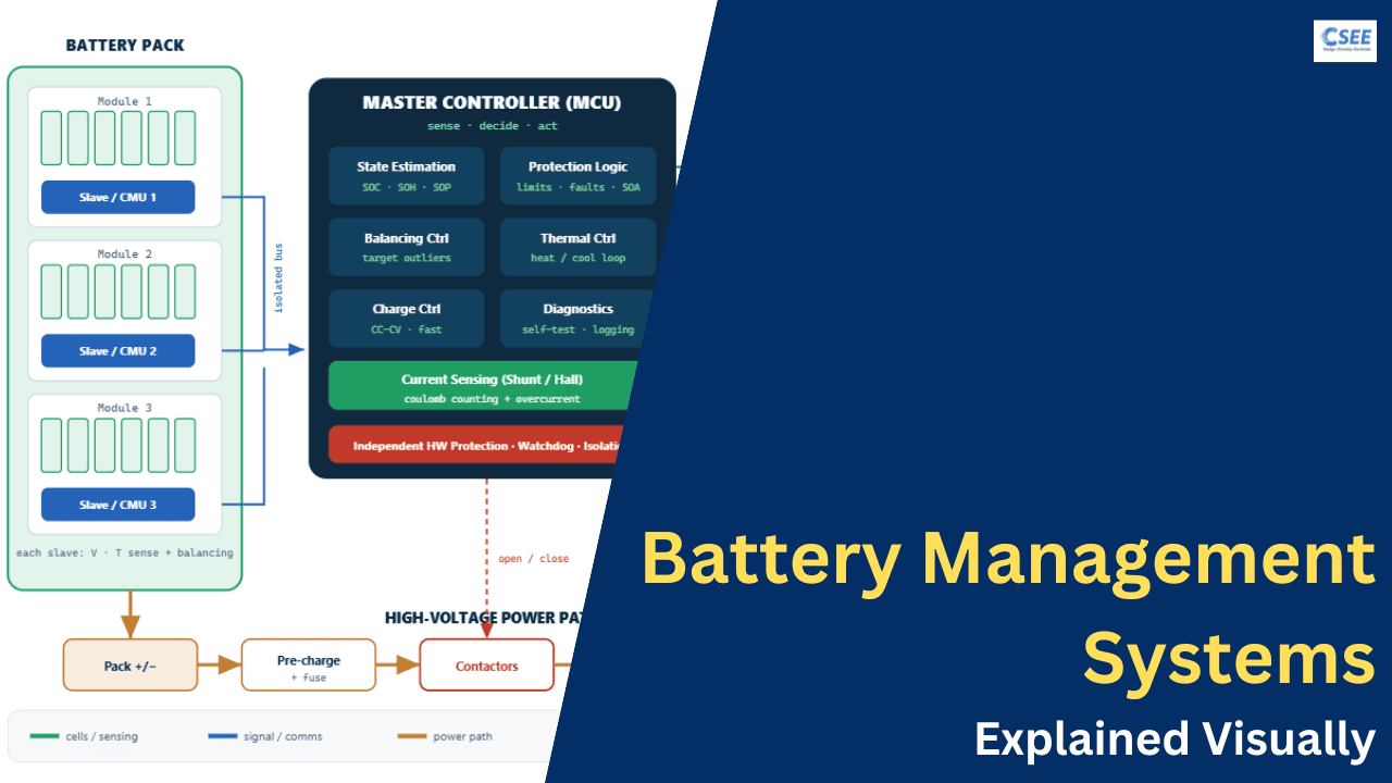
Before diving into any single subsystem, it helps to see the whole machine at once. The diagram below shows every major block of a modular battery management system and how signals, power, and decisions flow between them — the sensing front-ends on the cells, the master controller running the algorithms, the protection and power path, and the links to the outside world.
SECTION 01What a BMS is and why it exists
A Battery Management System (BMS) is the electronic control system that supervises a rechargeable battery pack. It measures what the cells are doing, decides what is safe, estimates quantities that cannot be measured directly, and acts to keep every cell inside a narrow window of voltage, current, and temperature for the entire life of the pack.
A single lithium-ion cell is a remarkable but unforgiving device. It stores a large amount of energy in a small, lightweight package, yet it tolerates almost no abuse. Charge it a few hundred millivolts too high and you plate metallic lithium onto the anode, permanently losing capacity and creating internal shorts. Discharge it too low and you dissolve the copper current collector. Push too much current when it is cold and you accelerate the same lithium plating. Let one cell run hot enough and it can enter thermal runaway, venting flammable gas and igniting its neighbours. The BMS exists because a bare battery pack is, without supervision, a hazard that also wears out quickly.
The problem multiplies with scale. A smartphone uses one cell. A power tool uses five to ten. An electric vehicle traction pack can contain anywhere from roughly one hundred to several thousand cells, wired in long series strings to reach hundreds of volts and in parallel groups to reach hundreds of amp-hours. In a series string, the weakest cell sets the limit: the pack can only be charged until the first cell reaches its ceiling, and only be discharged until the first cell hits its floor. Small differences in capacity, internal resistance, and self-discharge — differences that are inevitable in manufacturing and that grow with age — mean the cells drift apart over time. Without active management the usable capacity of the whole pack shrinks to that of its worst cell, and safety margins evaporate.
So the BMS has three jobs that recur throughout this tutorial, and it is worth fixing them in mind now:
- Protect. Keep every cell within its safe operating area for voltage, current, and temperature, and disconnect the pack before any limit is crossed.
- Estimate. Report how much charge remains (state of charge), how healthy the pack is (state of health), and how much power it can safely deliver right now (state of power) — none of which can be read off a meter directly.
- Optimise. Balance the cells, manage temperature, and control charging so the pack delivers the most usable energy and the longest life the chemistry allows.
Where the BMS sits in the system
The BMS is not the charger, and it is not the load. It is the intermediary that both of those must obey. A charger supplies current, but the BMS tells it when to stop or slow down. A motor inverter draws current, but the BMS tells the vehicle how much is available and can open the main contactors to cut everything off. In grid storage the same relationship holds between the power-conversion system and the racks of cells. This gate-keeper position is why the BMS is always the component that carries the highest safety rating in the system.
SECTION 02Cells, chemistry, and pack terminology
Before you can manage a battery you need a precise vocabulary for it. The words “cell”, “module”, and “pack” are not interchangeable, and the numbers that describe them drive every design decision downstream.
Cell, module, pack
A cell is the smallest complete electrochemical unit: two electrodes, a separator, and electrolyte in one enclosure, with a single positive and single negative terminal. A module is a mechanically and electrically grouped set of cells — often with its own sensing electronics — designed to be handled and serviced as a unit. A pack is the full assembly of modules plus the BMS, contactors, fuses, cooling, and enclosure that connects to the outside world. Series and parallel arrangement is written in the form xSyP: 96S2P, for example, means ninety-six cells in series, each “series position” actually being two cells in parallel, for a nominal voltage near 355 V and double the capacity of a single cell.
The parameters that matter
Every cell datasheet reduces to a handful of numbers that the BMS designer must respect. Nominal voltage is the rough average voltage over a discharge, used for labelling. Capacity, measured in amp-hours (Ah), is how much charge the cell holds; multiply by nominal voltage to get energy in watt-hours (Wh). C-rate expresses current as a multiple of capacity: a 1C current fully discharges a cell in one hour, 2C in half an hour, 0.5C in two hours. Internal resistance determines how much the terminal voltage sags under load and how much heat the cell generates. Finally, the manufacturer specifies hard limits — maximum and minimum voltage, maximum charge and discharge current at a given temperature, and an allowed temperature range — that define the box the BMS must never let a cell leave.
| Chemistry | Nominal V | Voltage window | Key strength | BMS implication |
|---|---|---|---|---|
| LFP (LiFePO₄) | 3.2 V | 2.5–3.65 V | Very safe, long cycle life | Extremely flat voltage curve makes SOC hard to read from voltage alone |
| NMC | 3.6–3.7 V | 3.0–4.2 V | High energy density | Steeper curve helps SOC; tighter thermal and overcharge margins |
| NCA | 3.6 V | 3.0–4.2 V | High energy, used in some EVs | Sensitive to overcharge; strong thermal monitoring needed |
| LTO (titanate) | 2.4 V | 1.5–2.8 V | Fast charge, wide temperature, long life | Lower cell voltage means more series cells for the same bus voltage |
| Lead-acid | 2.0 V | 1.75–2.4 V | Cheap, robust | Tolerant of overcharge; balancing less critical but still monitored |
Why cells drift apart
No two cells are identical. Manufacturing tolerances leave small spreads in capacity and resistance. In service, cells at different positions in the pack run at slightly different temperatures — the ones in the middle of a module stay warmer — and temperature strongly affects both aging rate and self-discharge. Over hundreds of cycles these small differences compound. A cell with slightly higher self-discharge slowly falls behind its neighbours in charge; a cell with slightly lower capacity reaches full and empty sooner. Left alone, the string’s usable range collapses to the intersection of every cell’s range. Managing this divergence is the job of balancing, covered in Section 09, and it is one of the clearest reasons a BMS earns its place.
SECTION 03BMS architectures
How you physically distribute the sensing and control electronics across a pack is one of the first and most consequential design decisions. Three canonical topologies exist — centralized, modular (master–slave), and distributed — and each trades cost, wiring, scalability, and reliability differently.
Centralized architecture
In a centralized BMS, a single electronic board contains everything: the microcontroller, the cell-measurement front-ends, the current sensor interface, the balancing circuitry, and the communication interface. Every cell tap wire runs from the pack back to this one board. This is the simplest and cheapest approach, and it is common in small packs — laptops, power tools, e-bikes, small energy-storage units — where the number of cells is modest and they are physically close together.
The weakness of the centralized approach is wiring. Each series connection needs its own sense wire back to the board, so a large pack becomes a nightmare of long, bundled, high-voltage harnessing that is heavy, error-prone to assemble, and vulnerable to noise and to a single connector failure taking out many measurements. Centralized designs therefore rarely scale past a few dozen cells in series.
Modular / master–slave architecture
The modular approach splits the sensing across several slave boards (also called cell-monitoring units or CMUs), each dedicated to a group of cells — typically one module. Each slave measures the voltages and temperatures of its local cells and handles their balancing, then reports over a communication link to a central master. The master runs the state-estimation algorithms, makes the protection decisions, drives the contactors, and talks to the rest of the system.
This is the dominant architecture in electric vehicles and large stationary storage. Because each slave sits next to its cells, sense wires stay short and local, and only a thin communication bus runs the length of the pack. Adding capacity is a matter of adding modules and slaves, so the design scales cleanly. The trade-off is more total electronics and a communication link that must itself be robust and isolated, since it may span hundreds of volts of potential difference between modules.
Distributed architecture
The distributed approach pushes electronics all the way down: a small monitoring circuit is integrated onto or into each cell or each series group, and only a communication bus and power leads run between them. This maximises wiring simplicity and gives per-cell diagnostics, but it multiplies the electronics count and cost. It appears in some high-end and aerospace packs and in emerging “smart cell” concepts.
| Attribute | Centralized | Modular (master–slave) | Distributed |
|---|---|---|---|
| Wiring complexity | High (all taps to one board) | Low (short local + one bus) | Lowest |
| Cost | Lowest | Moderate | Highest |
| Scalability | Poor | Excellent | Excellent |
| Diagnostics granularity | Pack-level | Module-level | Cell-level |
| Single-point failure impact | High | Contained to a module | Contained to a cell |
| Typical use | Tools, e-bikes, small ESS | EVs, grid storage | Aerospace, smart cells |
SECTION 04Hardware building blocks
Whatever the topology, the same functional blocks appear. Understanding each one — what it does and why it is hard — is the key to reading any BMS schematic.
The analog front-end (AFE)
The analog front-end, sometimes called the battery monitoring IC or cell supervisor, is the heart of the sensing chain. A single AFE typically monitors a stack of cells in series — commonly 6, 12, or 16 — measuring each cell’s voltage differentially against its neighbours, reading several temperature channels, and providing the switches used for balancing. The hard part is that the AFE must resolve a small per-cell voltage (a few volts) that sits on top of a large and varying common-mode voltage (the sum of all the cells below it, which can be hundreds of volts). It must do this to millivolt accuracy while rejecting noise, and it must survive hot-plugging and transient events. Modern AFEs achieve better than ±2 mV accuracy and include built-in diagnostics that check their own references and detect open sense wires.
The microcontroller
The microcontroller (MCU) runs the firmware: it schedules measurements, executes the state-estimation algorithms, enforces the protection logic, drives balancing, manages communication, and logs data. In a modular design the MCU lives on the master; in a centralized design it shares the board with the AFE. Safety-relevant designs use MCUs with hardware features that support fault detection — lockstep cores that run the same code twice and compare, memory protection, and watchdog timers that reset the system if the firmware stops responding.
Current sensing
Pack current is measured in one of two ways. A shunt resistor is a precise, very-low-value resistor placed in the main current path; the tiny voltage across it is proportional to current by Ohm’s law and is amplified and digitised. Shunts are accurate and cheap but dissipate heat and are galvanically connected to the current path. A Hall-effect sensor measures the magnetic field around the conductor and is inherently isolated, but it is more sensitive to temperature drift and external fields. Current measurement quality directly limits the accuracy of coulomb-counting, so this is not a place to economise.
Contactors, pre-charge, and fuses
The main contactors are the high-voltage relays that connect and disconnect the pack from the load. Because a large capacitive load would draw a destructive inrush current if connected instantly, a pre-charge circuit — a resistor in series with a smaller relay — first charges the load capacitance gently before the main contactor closes. A fuse provides a last-resort, purely physical interruption if current ever exceeds a catastrophic threshold faster than the electronics can react. Together these form the pack’s power-path safety layer.
Isolation and the isolated supply
In a high-voltage pack, the low-voltage control electronics and the human-facing interfaces must be galvanically isolated from the high-voltage domain. This is achieved with digital isolators, isolated communication transceivers, and isolated power supplies. A dedicated isolation monitor continuously checks the resistance between the high-voltage rails and chassis ground; a drop in that resistance signals insulation breakdown and is treated as a serious fault.
SECTION 05Measurement and sensing
Everything a BMS does rests on three measurements: cell voltage, pack current, and temperature. If these are wrong, every downstream decision and estimate is wrong. Sensing is therefore the discipline that most separates a good BMS from a mediocre one.
Cell voltage
Cell voltage is the single most important signal. It bounds charge and discharge directly — a cell must never be charged above its ceiling or discharged below its floor — and it feeds the state-of-charge estimate. The challenge is accuracy under difficult conditions. The measurement is differential and rides on a large common-mode voltage; it must remain accurate across the full temperature range and over years of aging; and it must reject the electrical noise of a high-current power system switching nearby. A specification of ±1 to ±5 mV is typical. To appreciate why that matters, note that near the flat middle of an LFP curve, a several-millivolt error can correspond to a large error in inferred state of charge.
Sense-wire integrity
A subtle but critical concern is the sense wire itself. If a tap wire develops resistance or breaks, the measured voltage becomes wrong or open, and the balancing current — which flows through the same wires in many designs — can create voltage offsets. Good AFEs include open-wire detection that periodically pulls a small current through each tap to confirm continuity, and firmware cross-checks the sum of cell voltages against the independently measured pack voltage.
Current
Current measurement feeds coulomb counting, power limiting, and overcurrent protection. The two dominant technologies — shunt and Hall-effect — were introduced in Section 04. The practical issues are offset and drift: a small zero-current offset, integrated over hours by a coulomb counter, becomes a large charge error. BMS firmware continually re-zeroes the current sensor during known rest periods and often uses two sensing ranges — a high-resolution channel for small currents and a wide channel for peak currents — because a single sensor cannot resolve milliamps and hundreds of amps at once.
Temperature
Temperature governs everything: allowable current, aging rate, balancing decisions, and the onset of thermal runaway. Because a pack cannot have a sensor on every cell, designers place thermistors at strategically chosen points — typically the locations expected to run hottest and coldest — and infer the rest. Temperature also feeds the electrochemical models used in advanced state estimation, since a cell’s resistance and available capacity both change strongly with temperature.
| Signal | Feeds | Typical target | Main error sources | Mitigation |
|---|---|---|---|---|
| Cell voltage | Limits, SOC, balancing | ±1–5 mV | Common-mode, noise, sense-wire resistance | Differential AFE, open-wire detection, sum cross-check |
| Current | Coulomb counting, power limits, OCP | ±0.5–1% | Offset, thermal drift, limited range | Rest re-zeroing, dual-range, temperature comp. |
| Temperature | Limits, aging, models | ±1–2 °C | Sparse placement, sensor lag | Worst-case placement, thermal modelling |
| Isolation resistance | Insulation fault detection | >100 Ω/V | Moisture, damage, aging | Continuous isolation monitor |
SECTION 06Core functions overview
With the hardware and signals established, we can enumerate what the firmware actually does. Every BMS, from a single-cell wearable to a megawatt storage container, implements some subset of these functions. The rest of the tutorial expands each of them.
| Function group | What it does | Covered in |
|---|---|---|
| Measurement | Acquire cell voltage, current, temperature, isolation | Section 05 |
| State estimation | Compute SOC, SOH, SOP, SOE | Sections 07–08 |
| Cell balancing | Equalise charge across the series string | Section 09 |
| Thermal management | Keep cells in their temperature window | Section 10 |
| Protection | Enforce voltage/current/temperature limits; open contactors | Section 11 |
| Communication | Report status, receive commands, log data | Section 12 |
| Charge control | Command charger, run CC–CV, manage fast charge | Section 13 |
| Diagnostics & safety | Detect faults, self-test, meet functional-safety targets | Sections 11, 14 |
A useful way to organise these in your mind is the sense–decide–act loop that appears on the BMS in this tutorial’s hero image. The BMS senses the pack (measurement), decides what is true and what is safe (estimation, protection logic, diagnostics), and acts on the world (balancing, thermal, charge control, contactors, communication). This loop runs continuously, at rates from a few hertz for slow thermal effects up to many kilohertz for fast protection paths.
SECTION 07State estimation: SOC, SOH, SOP, SOE
Here is the deep problem that makes battery management intellectually interesting: the quantities users care about most cannot be measured. You cannot put a probe on a cell and read its charge, its health, or its available power. They must be estimated from the measurable signals — voltage, current, temperature — through models of how the cell behaves.
State of charge (SOC)
State of charge is the fraction of usable capacity remaining, from 0% (empty) to 100% (full). It is the battery equivalent of a fuel gauge. But unlike fuel, charge does not sit in a tank you can look into; it is inferred. Two facts make this hard. First, the relationship between voltage and charge depends on temperature, current, and age. Second, that relationship can be nearly flat — as in LFP — so voltage alone is a poor indicator over much of the range. SOC estimation is therefore the central algorithmic challenge of a BMS, and Section 08 is devoted to it.
State of health (SOH)
State of health captures how much the battery has degraded relative to when it was new. It is usually expressed as present capacity divided by rated capacity, or as the increase in internal resistance. A pack at 80% SOH holds roughly four-fifths of its original charge and is often considered near the end of its automotive life, though it may serve years more in a less demanding “second-life” role. SOH changes slowly, over months and years, so it is estimated by observing trends rather than instantaneous values.
State of power (SOP)
State of power answers a real-time question: how much power can the pack safely source or sink right now, for the next few seconds, without any cell crossing a voltage or temperature limit? A cold, nearly full pack can accept little charge current; a warm, mid-charge pack can deliver a lot. SOP is what a vehicle uses to decide how aggressively it may accelerate or regeneratively brake. It depends on SOC, temperature, internal resistance, and the cell limits, and it must be recomputed continuously.
State of energy (SOE)
State of energy is the energy analogue of SOC — the fraction of usable energy (watt-hours) remaining, as opposed to charge (amp-hours). Because a cell’s voltage falls as it discharges, energy and charge are not linearly related, and SOE gives a more accurate picture of usable range for an application whose consumption is measured in energy, such as predicting how many kilometres an EV can still travel.
| State | Question it answers | Units | Timescale |
|---|---|---|---|
| SOC — charge | How full is it now? | % of capacity (Ah) | Seconds–minutes |
| SOE — energy | How much range is left? | % of energy (Wh) | Seconds–minutes |
| SOP — power | How hard can I push it now? | Watts (charge/discharge) | Milliseconds–seconds |
| SOH — health | How worn out is it? | % capacity or % resistance | Months–years |
SECTION 08SOC and SOH algorithms in depth
This is the intellectual heart of a modern BMS. We will build up from the simplest, most intuitive method to the model-based estimators used in production electric vehicles, showing how each fixes the weakness of the one before.
Method 1 — Coulomb counting (charge integration)
The most direct idea is to count charge in and out. If you know the current at every instant, you can integrate it over time to track how much charge has entered or left the pack. Starting from a known state of charge, the current state is simply the starting value plus the accumulated charge divided by the capacity.
Here I is the current (positive on discharge), Cn is the usable capacity in amp-seconds, and η is coulombic efficiency, a factor slightly below 1 that accounts for the small fraction of charge lost to side reactions. Coulomb counting is simple, works for any chemistry including flat-curve LFP, and responds instantly to load. Its fatal flaw is drift: any error in the current measurement, however small, is integrated forever. A tiny current offset accumulates into a growing charge error, and the initial SOC(t0) must be known from somewhere. Coulomb counting alone is accurate over minutes but untrustworthy over days.
Method 2 — Open-circuit voltage (OCV) lookup
Every cell chemistry has a characteristic relationship between its rested, open-circuit voltage and its state of charge. If you let a cell relax with no load until its voltage settles, that settled voltage maps to a unique SOC through a calibration curve. This method needs no integration and does not drift, which makes it the perfect complement to coulomb counting.
OCV lookup has two weaknesses. First, it requires rest — the cell must relax for minutes to hours after a load before the voltage truly settles, so it cannot be used continuously while the pack is working. Second, as Figure 8.1 shows, on a flat chemistry the curve provides almost no resolution in the middle. Real systems therefore use OCV opportunistically: whenever the pack has rested (for example, a car parked overnight), the BMS reads OCV, converts it to SOC, and uses it to re-anchor the drifting coulomb counter.
Method 3 — Equivalent-circuit models
To use voltage during operation, we need to account for the cell’s dynamic response. Under load, a cell’s terminal voltage differs from its OCV because of internal resistance and slower diffusion effects. An equivalent-circuit model (ECM) captures this with a voltage source (the OCV, a function of SOC) in series with an ohmic resistance and one or more resistor–capacitor (RC) pairs that model the transient relaxation.
With such a model, if you know the parameters (R0, R1, C1, and the OCV curve) you can predict terminal voltage from current and SOC. Invert the logic and you can infer SOC from measured voltage and current — but only if the model is accurate, and the parameters themselves drift with temperature and age. This sets up the final step: fuse the model prediction with the measurement, weighting each by how much you trust it. That is exactly what a Kalman filter does.
Method 4 — Kalman filtering (EKF / UKF)
The Kalman filter is a recursive estimator that optimally combines a model’s prediction with a noisy measurement. It maintains not just a best estimate of the state but also a measure of its uncertainty. Each cycle has two phases. In the predict phase, the model (coulomb counting plus the RC dynamics) projects the state forward and the uncertainty grows. In the update phase, the measured terminal voltage is compared to what the model predicted; the difference — the “innovation” — corrects the state, and the uncertainty shrinks. The relative trust given to model versus measurement is the Kalman gain, computed automatically from the uncertainties.
Because a battery is nonlinear (the OCV–SOC relationship is a curve, not a line), the plain Kalman filter does not apply directly. Two nonlinear variants dominate: the Extended Kalman Filter (EKF), which linearises the model at each step, and the Unscented Kalman Filter (UKF), which propagates a small set of carefully chosen sample points through the true nonlinear model for better accuracy without derivatives. Both are workhorses of production EV battery management.
In pseudocode, a single EKF cycle for SOC looks like this:
# state x = [SOC, V1];  inputs: current I, measured voltage Vmeas, dt
function ekf_step(x, P, I, Vmeas, dt):
    # --- 1. PREDICT ---
    SOC   = x.SOC - eta * I * dt / Cn          # coulomb counting
    V1    = x.V1  * exp(-dt/(R1*C1)) + I*R1*(1 - exp(-dt/(R1*C1)))
    x_pred = [SOC, V1]
    P      = F * P * F.T + Q                    # grow uncertainty

    # --- 2. UPDATE ---
    V_pred = OCV(SOC) - I*R0 - V1           # model output
    y      = Vmeas - V_pred                     # innovation
    H      = [dOCV/dSOC, -1]                    # linearise
    K      = P * H.T / (H * P * H.T + Rnoise)   # Kalman gain
    x      = x_pred + K * y                     # correct estimate
    P      = (I_mat - K * H) * P                # shrink uncertainty
    return x, P
Method 5 — Data-driven and hybrid approaches
Machine-learning methods — neural networks, in particular recurrent architectures suited to time series — can learn the mapping from measured signals to SOC or SOH directly from large datasets, capturing nonlinearities and aging effects that are hard to model by hand. In practice they are usually combined with the physics-based estimators rather than replacing them: a model-based filter provides a robust, explainable backbone, while learned components correct for effects the model misses. Pure black-box estimators are used cautiously in safety-critical systems because their behaviour outside the training distribution is hard to guarantee.
| Method | Idea | Strength | Weakness | Where used |
|---|---|---|---|---|
| Coulomb counting | Integrate current | Simple, instant, any chemistry | Drifts; needs a starting point | Everywhere, as a backbone |
| OCV lookup | Rested voltage → SOC | No drift, self-anchoring | Needs rest; poor on flat curves | Re-anchoring after rest |
| ECM + observer | Model dynamic voltage | Works under load | Parameters drift with age/temp | Basis for filters |
| EKF / UKF | Fuse model + measurement | Robust, tracks uncertainty | Tuning effort, compute cost | Production EVs |
| Machine learning | Learn mapping from data | Captures complex aging | Needs data; hard to certify alone | Hybrid, research, cloud analytics |
Estimating state of health
SOH estimation watches long-term trends. Capacity fade is measured by tracking how much charge actually flows between two well-known SOC anchor points — if a full charge from a known-empty to a known-full state now passes less charge than it did when new, capacity has faded. Resistance growth is measured from the voltage response to current steps: an aged cell shows a larger voltage sag for the same current. Advanced systems also use incremental capacity analysis, which examines the shape of the charge–voltage curve for features that shift characteristically as specific degradation mechanisms progress. Because these signals are slow and noisy, SOH is filtered heavily and updated over many cycles rather than in real time.
DEEP DIVEWorked examples: making the numbers concrete
Formulas are easier to trust once you have pushed real numbers through them. This section works three small calculations by hand — coulomb counting, a state-of-power limit, and a balancing time — so the abstractions of the previous sections turn into something you can feel.
Example 1 — How fast does coulomb counting drift?
Suppose a pack has a usable capacity of 100 Ah and a current sensor with a small, unnoticed zero offset of 50 mA — a fraction of a percent of its full range, easy to miss. The coulomb counter integrates that phantom current continuously. Over one hour it accumulates 50 mA × 1 h = 50 mAh of error. Divided by the 100 Ah capacity, that is 0.05% of state of charge per hour. That sounds negligible, and over a short drive it is. But leave the pack sitting for a week and the same offset accumulates 50 mA × 168 h = 8.4 Ah — an 8.4% state-of-charge error from nothing but a tiny, constant sensor bias. This single arithmetic is the whole argument for re-anchoring the counter from open-circuit voltage whenever the pack rests, and it explains why current-sensor offset calibration is treated so seriously.
Example 2 — What limits discharge power right now?
State of power asks how much current the pack can deliver before the weakest cell hits its voltage floor. Take a cell currently resting at an open-circuit voltage of 3.5 V with an internal resistance of 20 mΩ, and a discharge floor of 3.0 V. Under load the terminal voltage sags by the current times the resistance. The maximum current is the one that just brings the terminal voltage down to the floor:
So this cell can supply about 25 A this instant. Note what happens as the pack ages: internal resistance grows, say to 40 mΩ, and the same calculation yields only 12.5 A. The pack’s deliverable power falls even though its stored charge is unchanged — which is exactly why state of power and state of health must be tracked separately from state of charge, and why an old pack feels weak under load long before it feels empty. In practice the BMS also folds in temperature (which changes R₀) and a safety margin, and recomputes this every control cycle.
Example 3 — How long does passive balancing take?
Imagine one cell holds 200 mAh more charge than its neighbours and the passive bleed resistor draws 100 mA when switched on. Ignoring the small trickle the cell keeps receiving, the time to burn off the surplus is simply the excess charge divided by the bleed current: 200 mAh ÷ 100 mA = 2 hours. This is why passive balancing is slow and is spread across many charge cycles rather than completed in one sitting, and why designers keep cell mismatch small in the first place — every reclaimed milliamp-hour costs balancing time and is dissipated as waste heat.
DEEP DIVEHow batteries age — the mechanisms behind SOH
State of health is a number, but behind it are physical processes slowly consuming the cell. Understanding them explains why the BMS makes the choices it does about temperature, charge limits, and depth of discharge — and why those choices extend a pack’s life.
Calendar aging versus cycle aging
A battery degrades in two distinct ways. Calendar aging happens simply with the passage of time, whether or not the pack is used, and is driven mainly by temperature and by the state of charge at which the cell sits. A cell stored hot and full ages far faster than one stored cool and partly charged — which is why manufacturers recommend storing packs at a moderate state of charge and why an EV left in the sun at 100% for months loses more health than one parked cool at 60%. Cycle aging happens as a consequence of charging and discharging, and depends on how deeply the cell is cycled, how fast, and again how hot. Shallow cycles around the middle of the range are gentle; deep, fast cycles to both extremes are harsh.
What actually degrades
At the electrode level, several mechanisms compound. The most important in most lithium-ion cells is growth of the solid–electrolyte interphase, a passivating layer on the anode that forms naturally but continues to thicken over life, consuming lithium and electrolyte and raising internal resistance. Lithium plating — metallic lithium depositing on the anode instead of intercalating into it — occurs during charging that is too fast or too cold, permanently locking away lithium and, in the worst case, forming dendrites that can pierce the separator. Active-material loss from mechanical stress as the electrodes repeatedly expand and contract, and electrolyte decomposition at high voltage and temperature, round out the picture. The visible symptoms of all of this are the two things the BMS tracks: capacity fade and resistance growth.
| Driver | Effect | BMS mitigation |
|---|---|---|
| High temperature | Accelerates all side reactions | Cooling; limit power when hot |
| High state of charge held long | Faster calendar aging | Recommend/enforce lower storage SOC |
| Deep discharge to the floor | Electrode stress, capacity loss | Conservative usable window |
| Fast or cold charging | Lithium plating | Limit charge current; pre-heat; SOP control |
| High cycle count / throughput | Cumulative wear | Efficient use; accurate SOH to plan life |
This is why so much of the BMS’s optimisation work is really life-extension work in disguise. Every time it caps a fast charge on a cold morning, holds a lower storage charge, keeps the pack cool, or refuses the last few percent of the voltage range, it is trading a small amount of immediate performance for a large amount of future capacity. The state-of-health estimate closes the loop: by measuring how the pack is actually aging, the BMS can verify that its strategies are working and can tell the user, honestly, how much life remains.
SECTION 09Cell balancing
Recall from Section 02 that cells in a series string inevitably drift apart, and that the weakest cell caps the whole string. Balancing is the process of deliberately redistributing or removing charge so that every cell reaches full and empty together, reclaiming the capacity that divergence would otherwise waste.
Passive balancing
Passive balancing is the simpler and far more common approach. Each cell has a bleed resistor that can be switched across it. When a cell runs ahead of the others — reaching a higher voltage during charge — the BMS turns on that cell’s resistor, dissipating its excess charge as heat until it falls back in line with the rest. The result is that all cells finish charging at the same level. Passive balancing only ever removes charge, so it can only bring the stronger cells down to the weakest; it cannot lift a lagging cell up. It is cheap, compact, and reliable, and it dominates consumer and automotive designs where cell matching is good and the balancing currents needed are small.
Active balancing
Active balancing moves charge from stronger cells to weaker ones instead of wasting it, using energy-storage elements — capacitors, inductors, or small transformers — as intermediaries. A charge is scooped from a high cell and delivered to a low cell, so nothing is thrown away and a lagging cell can actually be lifted up. This recovers more usable capacity and produces less heat, which matters in large packs, but it costs far more components, board area, and control complexity. Active balancing appears where the value of every reclaimed watt-hour is high or where cells are poorly matched, such as some large stationary systems and second-life packs.
| Aspect | Passive | Active |
|---|---|---|
| Mechanism | Bleed excess to heat | Transfer charge between cells |
| Direction | Only lowers high cells | Can raise low cells too |
| Efficiency | Low (energy wasted) | High (energy conserved) |
| Cost & complexity | Low | High |
| Heat generated | Higher | Lower |
| Typical use | Consumer, most EVs | Large ESS, second-life, mismatched cells |
When to balance
Balancing is usually most effective near the top of charge, where the OCV curve is steep and small charge differences produce readable voltage differences — this is especially true for LFP, whose flat middle hides imbalance entirely. Many BMSs balance during charging and during rest, and pause balancing during heavy discharge to avoid confusing the current measurement. The BMS decides which cells to balance by comparing each cell’s voltage (or, better, its estimated SOC) against the pack and targeting the outliers.
SECTION 10Thermal management
Temperature is the variable that most strongly governs both performance and life. Every cell has a narrow band — very roughly 15 to 35 °C — where it works best. Outside it, capability, safety, and longevity all suffer, and the BMS is responsible for keeping the pack inside that band.
Why temperature matters so much
Cold cells have high internal resistance, so they deliver and accept less power, and charging a cold cell risks lithium plating that permanently damages it — which is why an EV may refuse or slow fast charging in winter until the pack warms. Hot cells age faster: the chemical side reactions that consume capacity roughly double in rate for every ten-degree rise, so a pack run persistently hot wears out in a fraction of the cycles it would otherwise achieve. And beyond a critical temperature lies thermal runaway, the self-sustaining reaction the entire safety design exists to prevent.
Heating and cooling strategies
Thermal management ranges from passive to elaborate. The simplest packs rely on natural convection and thermal mass. Air cooling forces air across the cells with fans. Liquid cooling circulates a coolant through cold plates in contact with the cells, giving far better and more uniform heat removal — the standard in performance EVs. In cold climates, packs add heaters, sometimes routing waste heat from other systems, to bring cells into range before high power is allowed. The BMS commands all of this based on measured temperatures and on predicted heat generation from the current and the cells’ resistance.
SECTION 11Protection and fault handling
Protection is the function that justifies the BMS’s existence and its high safety rating. It is the set of always-on checks that keep every cell inside its safe operating area and that disconnect the pack the moment a limit is threatened.
The safe operating area
Every cell must stay inside a three-dimensional box defined by voltage, current, and temperature. Cross any face of that box and damage or danger follows. The BMS enforces the box with layered limits: a warning level that de-rates performance and alerts the system, and a hard level that opens the contactors. Crucially, the fastest and most dangerous events — a dead short, for instance — are handled by dedicated hardware that acts in under a millisecond, faster than firmware could respond, with the microcontroller providing the slower, smarter supervisory layer on top.
The main protection faults
| Fault | Trigger | Risk if ignored | Typical response |
|---|---|---|---|
| Cell over-voltage | Any cell above ceiling during charge | Lithium plating, overheating, runaway | Stop/slow charge; open contactor |
| Cell under-voltage | Any cell below floor during discharge | Copper dissolution, permanent damage | Stop discharge; open contactor |
| Over-current (charge/discharge) | Current beyond limit | Overheating, cell damage | De-rate, then open contactor; fuse as last resort |
| Over-temperature | Any sensor above limit | Accelerated aging, runaway | De-rate, cool, then disconnect |
| Under-temperature charge | Charging below allowed temp | Lithium plating | Block charge; heat pack first |
| Short circuit | Sudden extreme current | Fire | Hardware trip in <1 ms; fuse |
| Isolation loss | HV-to-chassis resistance drops | Shock hazard | Warn; disconnect depending on severity |
| Sensor / comms fault | Implausible or missing data | Blind operation | Enter safe state; limit or disconnect |
Plausibility and self-diagnosis
A protection system is only as trustworthy as its own health. A BMS therefore does not merely act on its readings — it constantly checks that those readings make sense. It cross-checks the sum of cell voltages against the pack voltage, verifies that current and voltage changes are consistent, watches for sensor values that jump impossibly fast, and confirms that each measurement channel is alive. If the data becomes untrustworthy, the safe response is to assume the worst and move the pack toward a safe state rather than to trust a possibly-faulty reading. This philosophy — fail safe, not fail operational — runs through the functional-safety standards discussed in Section 14.
SECTION 12Communication interfaces
A BMS is never an island. Internally, slaves must talk to the master; externally, the master must report to the vehicle, the charger, or the grid controller. The communication layer carries the pack’s status outward and commands inward, and in safety systems it must itself be robust, isolated, and diagnosable.
Internal communication
Inside the pack, the master and slaves communicate over one of two common schemes. A daisy-chain links each slave to the next in a vertical stack, passing data up and down through isolated links; it minimises wiring and is designed to bridge the large voltage differences between modules. Alternatively, an isolated internal CAN bus connects all slaves as peers to the master. Lower-level chip-to-chip links such as SPI and I²C appear on individual boards between the microcontroller and its front-end and memory devices.
External communication
To the outside world, the CAN bus — and its higher-bandwidth successor CAN FD — is the near-universal automotive choice: robust, deterministic, and designed for noisy vehicle environments. In grid and industrial storage, protocols such as Modbus and various Ethernet-based industrial protocols are common. Charging brings its own standardised messaging so the pack and charger can negotiate voltage and current safely; the BMS is an active participant in this negotiation, not a passive recipient of whatever the charger provides.
| Interface | Where | Character |
|---|---|---|
| SPI / I²C | MCU ↔ AFE / memory, on-board | Fast, short-range, chip-to-chip |
| Isolated daisy-chain | Master ↔ slaves across HV stack | Minimal wiring, isolated per link |
| Internal CAN | Master ↔ slaves | Robust multi-node bus |
| CAN / CAN FD | Pack ↔ vehicle / charger | Automotive standard, deterministic |
| Modbus / Ethernet | Pack ↔ grid / industrial controller | Stationary storage, monitoring |
SECTION 13Charging control
Charging is where the BMS is most actively in command. It does not simply allow current to flow; it dictates the profile, moment to moment, that keeps every cell safe while filling the pack as quickly as the chemistry permits.
Constant current, constant voltage (CC–CV)
The standard lithium-ion charge profile has two phases. In the constant-current (CC) phase, the charger pushes a steady current and the cell voltage climbs. Once the voltage reaches the ceiling, the profile switches to the constant-voltage (CV) phase: the voltage is held at the ceiling and the current is allowed to taper naturally as the cell fills, until the current falls below a small cutoff and charging ends. The CC phase does the bulk of the work quickly; the CV phase tops off the last portion gently, because forcing more current at high voltage would overshoot the limit and damage the cell.
Fast charging and temperature
Fast charging pushes the CC current high to fill the pack in minutes rather than hours, but the higher the current, the more heat is generated and the closer the cells run to their plating and thermal limits. The BMS manages this by continuously computing the maximum current each cell can accept — its charge-direction state of power — and commanding the charger to stay under it. Because cold cells plate lithium under fast charge, the BMS may pre-heat the pack before allowing full-rate charging, and it de-rates the current as any cell or sensor approaches a temperature limit. The result is a charge curve that is aggressive when conditions allow and cautious when they do not, all managed transparently to the user.
SECTION 14Functional safety and standards
Because a BMS failure can cause fire, injury, or death, battery management is a functional-safety discipline. That means the system is engineered not just to work, but to fail in predictable, safe ways, and to prove — through process and documentation — that its risk of dangerous failure is acceptably low.
Failing safe
The guiding principle is that when something goes wrong — a sensor dies, the firmware hangs, a communication link drops — the system must move to a defined safe state rather than continuing blindly. For a battery pack the safe state is usually “disconnected”: open the contactors and remove the hazard. Techniques that support this include redundant measurements that cross-check each other, watchdog timers that reset a stalled processor, lockstep processor cores that run the same computation twice and compare results, and independent hardware protection that acts even if the software fails entirely. The philosophy of Section 11 — assume the worst when data is untrustworthy — is the everyday expression of failing safe.
Safety integrity levels
Automotive functional safety is governed by the ISO 26262 standard, which classifies each hazard by an Automotive Safety Integrity Level (ASIL), from A (least stringent) to D (most stringent). The functions that can cause the most severe harm and are hardest for a driver to control — such as preventing an overcharge that could lead to a fire — are assigned the highest levels and must meet the most rigorous design, verification, and diagnostic-coverage requirements. Achieving a high ASIL shapes the entire architecture: it drives the redundancy, the self-tests, and the independent protection paths described throughout this tutorial.
| Standard | Domain | Concern |
|---|---|---|
| ISO 26262 | Automotive | Functional safety; ASIL classification of electronic systems |
| IEC 62619 | Industrial / stationary | Safety of secondary lithium cells and batteries |
| UL 1973 / UL 9540 | Stationary storage | Battery and energy-storage-system safety |
| UN 38.3 | Transport | Safety testing for shipping lithium batteries |
| ISO 6469 | Electric vehicles | Electrical safety of the on-board energy system |
SECTION 15Applications
The same core ideas scale across a huge range of products, but the emphasis shifts. Understanding how the priorities change from one application to another is a good test of whether the fundamentals have clicked.
Electric vehicles
The EV is the most demanding mainstream application. A traction pack combines hundreds of cells at hundreds of volts and must deliver both accurate range prediction and split-second power decisions while meeting the highest functional-safety levels. Its BMS is almost always modular, runs sophisticated model-based state estimation, manages liquid cooling and pre-heating, negotiates fast charging, and integrates deeply with the vehicle over CAN. Every theme in this tutorial appears here at full intensity.
Consumer electronics and power tools
At the small end, a phone or a cordless drill uses a handful of cells and a compact, often centralized or single-chip BMS. Safety and cycle life still matter, but the pack is small, the currents are modest, and cost and size dominate the design. State-of-charge accuracy is important because it feeds the battery icon the user watches, but the algorithms can be lighter than an EV’s.
Grid and stationary storage
Stationary storage runs from home batteries to container-scale installations that stabilise the electricity grid. Here the pack may cycle shallowly but constantly for a decade or more, so longevity and precise SOH tracking are paramount, and the sheer number of cells makes robust modular or distributed architectures and strong communication essential. Because these systems sit in buildings and substations, their safety and fire standards are stringent, and active balancing is more attractive because reclaimed energy is directly monetisable over a long life.
Second-life and specialised systems
Retired EV packs, still holding most of their capacity, find second lives in stationary storage. These packs contain cells that have aged unevenly, so their BMS must handle wider spreads in capacity and resistance, making accurate per-cell estimation and capable balancing especially valuable. Aerospace, medical, and marine systems add their own extreme reliability and certification requirements on top of everything covered here.
| Application | Cells | Dominant priority | Typical architecture |
|---|---|---|---|
| Electric vehicle | 100s–1000s | Safety, range accuracy, fast charge | Modular, liquid-cooled |
| Consumer / tools | 1–10 | Cost, size, basic safety | Centralized / single-chip |
| Grid storage | 1000s+ | Longevity, SOH, uptime | Modular / distributed |
| Second-life | 100s+ | Handling mismatch | Modular, strong balancing |
SECTION 16Design trade-offs and validation
Designing a BMS is an exercise in balancing competing goals under real constraints. No design is optimal on every axis; the craft is in choosing which compromises the application can afford.
The central trade-offs
Accuracy costs money and power: a more precise front-end, a wider-range current sensor, and more temperature channels all improve estimation but add cost and drain the very battery they measure. Safety adds redundancy, and redundancy adds components, weight, and expense. Active balancing recovers energy but multiplies part count. A more elaborate estimator improves range prediction but needs a more capable processor and far more engineering effort to tune and validate. Every one of these is a slider the designer sets according to the application’s priorities from Section 15.
| Lever | Buys you | Costs you |
|---|---|---|
| Higher sensing accuracy | Better estimates, tighter limits | Cost, power, complexity |
| Redundancy | Higher safety integrity | Parts, weight, cost |
| Active balancing | Recovered energy, less heat | Components, board area |
| Advanced estimation | Range accuracy, robustness | Compute, tuning, validation |
| Modular architecture | Scalability, serviceability | More electronics, a bus to secure |
Validating a BMS
Because you cannot ethically discover a safety flaw in the field, a BMS is validated exhaustively before deployment. Hardware-in-the-loop testing connects the BMS to a real-time simulator that emulates a battery pack, letting engineers rehearse thousands of fault scenarios — a broken sense wire, a stuck contactor, an implausible sensor — safely and repeatably. Cells are cycled through their whole life in accelerated aging tests to confirm that SOH estimation tracks reality and that limits hold as cells degrade. Abuse tests — overcharge, short circuit, crush, and thermal — verify that the protection layers behave as designed at the true edges. Only after this campaign, layered on top of the functional-safety process of Section 14, does a design earn its place in a product.
SECTION 17Future directions
Battery management is advancing quickly, pushed by the growth of electrified transport and grid storage. Several threads are reshaping what a BMS is and where its intelligence lives.
Cloud-connected and digital-twin management moves part of the analytics off the pack. By streaming operating data to a server that runs a detailed simulation model of each pack — a digital twin — fleets can refine SOH estimates, predict failures before they happen, and improve the on-board algorithms over the air. The pack keeps a robust local BMS for real-time safety while the cloud handles the slow, data-hungry learning.
Physics-based and machine-learning fusion continues to mature. Higher-fidelity electrochemical models, once too heavy to run on an embedded processor, are being reduced and combined with learned corrections to estimate not just charge and health but the internal states that predict aging and even the early signatures of a cell heading toward failure.
Smart cells and wireless BMS rethink the wiring itself. Integrating monitoring into each cell and replacing the sense harness with a wireless link inside the pack can cut weight and assembly complexity and improve per-cell diagnostics — at the cost of new challenges in wireless reliability and security. New chemistries, from silicon-rich anodes to solid-state and sodium-ion cells, each bring different voltage curves, thermal behaviour, and failure modes, and each will demand that the estimation and protection strategies covered here be re-tuned rather than reused wholesale.
Finally, as packs proliferate, sustainability is becoming a first-class BMS concern: the same health data that keeps a pack safe also determines whether it can be reused in a second life or must be recycled, and richer lifetime records make that decision cleaner. The BMS is increasingly the custodian of a battery’s entire life story, not just its present moment.
SECTION 18Glossary
A quick reference to the recurring terms in this tutorial.
| Term | Meaning |
|---|---|
| AFE | Analog front-end; the IC that measures cell voltages and temperatures and switches balancing. |
| ASIL | Automotive Safety Integrity Level (A–D); the risk classification from ISO 26262. |
| C-rate | Current expressed as a multiple of capacity; 1C empties the cell in one hour. |
| Cell / module / pack | The smallest unit; a serviceable group of cells; the full assembly with BMS and enclosure. |
| Contactor | High-voltage relay that connects or disconnects the pack. |
| Coulomb counting | Estimating charge by integrating current over time. |
| ECM | Equivalent-circuit model; a resistor–capacitor model of a cell’s voltage behaviour. |
| EKF / UKF | Extended / Unscented Kalman Filter; nonlinear estimators used for SOC. |
| OCV | Open-circuit voltage; a rested cell’s voltage, which maps to SOC. |
| Pre-charge | Gently charging the load capacitance before closing the main contactor. |
| SOA | Safe operating area; the box of allowed voltage, current, and temperature. |
| SOC / SOE | State of charge (Ah) / state of energy (Wh) remaining. |
| SOH | State of health; how degraded the pack is versus new. |
| SOP | State of power; how much power can safely be sourced or sunk right now. |
| Thermal runaway | A self-heating chain reaction that can destroy a cell and ignite its neighbours. |
| xSyP | Notation for x cells in series, y in parallel. |
IN CLOSINGBringing it together
A battery management system is the answer to a hard truth: lithium-ion cells store enormous energy but tolerate almost no abuse, and a series string is only as strong as its weakest member. From that truth everything in this tutorial follows. The BMS senses every cell to millivolt accuracy, decides what is true and safe by estimating charge, health, and power it cannot directly measure, and acts on the pack through balancing, thermal control, charge management, and — when a limit is threatened — decisive disconnection.
The estimation problem gives the field its intellectual depth: coulomb counting is instant but drifts, open-circuit voltage is stable but needs rest, and only by fusing a cell model with live measurements in a Kalman filter do you get an estimate that is both responsive and trustworthy. The safety problem gives the field its discipline: the entire architecture — redundancy, self-diagnosis, independent hardware protection, and the habit of failing safe — exists so that when something breaks, the pack becomes harmless rather than dangerous.
Master those two ideas — estimate what you cannot measure and fail toward safety — and every architecture, algorithm, circuit, and standard in the preceding eighteen sections falls into place as a different expression of the same goal: to make a demanding, unforgiving energy source safe, accurate, and long-lived enough to power the world.