Field Manual · Rev 2.0 · 10 Phases · ~8 Months
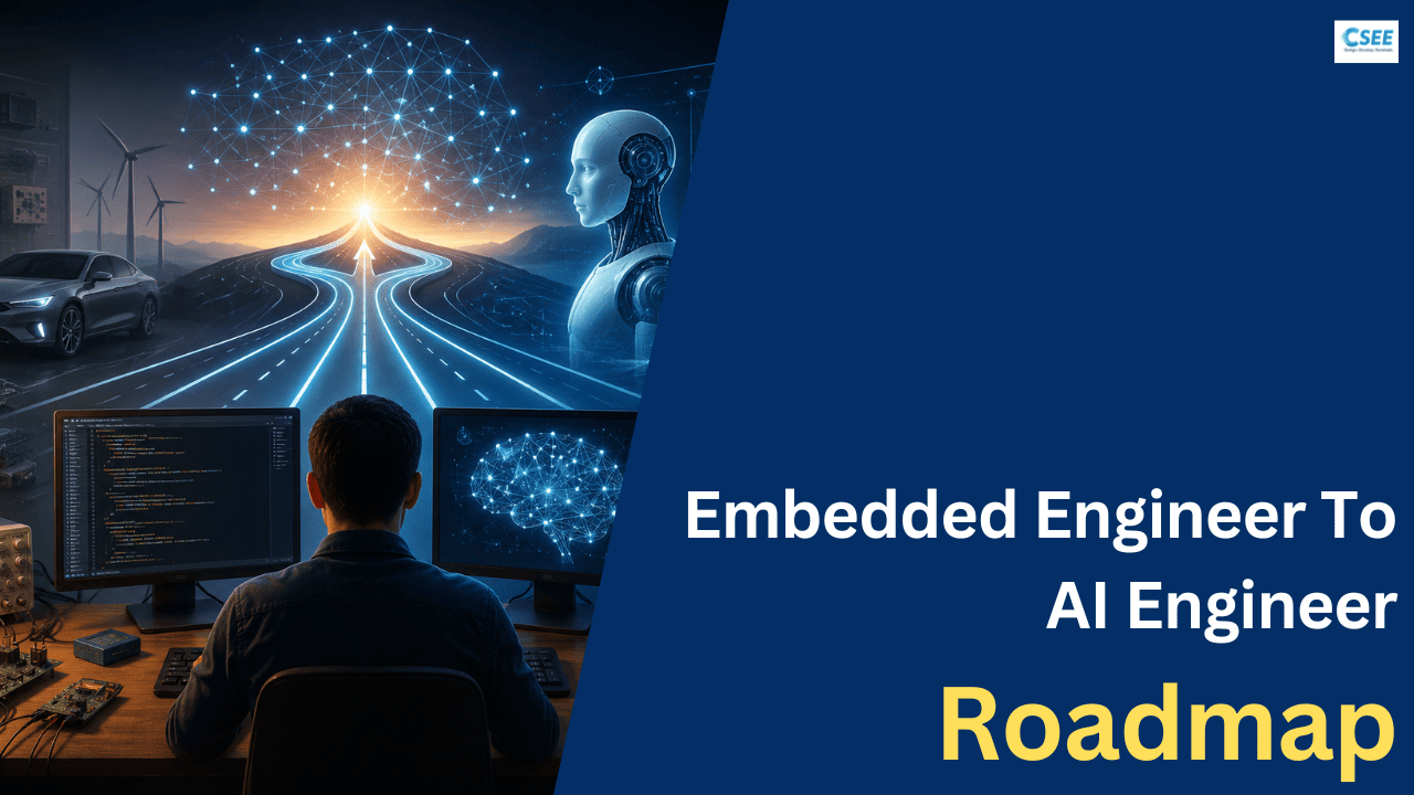
Embedded Engineer → AI Engineer
A phase-by-phase roadmap for engineers coming from firmware, RTOS, drivers, sensors and hardware bring-up — ending in Edge AI, MLOps and applied AI roles across robotics, industrial, consumer and automotive.
Your background is the shortcut, not the handicap
Before the ten phases, understand what you are carrying in. It changes what you study, in what order, and how you should describe yourself when you apply.
The popular image of an AI engineer is someone deriving gradients on a whiteboard. The reality of paid AI work is systems work: moving data from where it is to where it needs to be, keeping behaviour stable as inputs drift, fitting inference inside a latency budget, quantising a network so it survives on a device with half a megabyte of usable RAM, and building the observability that tells you when any of that has silently broken.
An engineer who has shipped firmware that runs unattended for years, chased an intermittent bus fault across three boards, or written the validation evidence for a release already thinks that way. What you are missing is statistics, a Python-centred toolchain, and a tolerance for non-determinism. Those are additions to a foundation, not a restart.
| What you do today | What it becomes in AI | Transfer strength |
|---|---|---|
| Embedded C, memory maps, DMA | Tensor memory layout, arena allocation, KV-cache sizing | Direct — same reasoning, new names |
| Fixed-point arithmetic, Q formats | INT8/INT4 quantisation, scale & zero-point, saturation | Direct — you already own this |
| Cycle counting, timing analysis | Inference latency budgets, throughput, batching | Direct |
| Control loops and state machines | Training loops, feedback, convergence and stability intuition | Strong — a training run behaves like a tuned loop |
| State estimation, filtering, calibration | Time-series regression, uncertainty, sensor modelling | Strong — these are already ML problems in disguise |
| Protocol and device log analysis | Log mining, anomaly detection, intrusion detection | Strong — and rare among ML candidates |
| V&V, HIL rigs, regression suites | Evaluation harnesses, golden datasets, CI for models | Strong — badly under-supplied in AI teams |
| Safety and reliability engineering | Guardrails, fallback paths, graceful degradation | Strong — a genuine differentiator for safety-adjacent AI |
| Signal conditioning, filtering, FFT | Feature engineering on sensor time-series | Strong |
| Probability and statistics | Loss functions, metrics, confidence, calibration | Partial — rebuild deliberately in Phase 2 |
| Deterministic debugging | Stochastic experiments, seeds, run-to-run variance | Weak — the biggest mental shift ahead of you |
Scroll table horizontally →
You are not competing with fresh graduates for generic ML jobs. You are aiming at the intersection — Edge AI, industrial AI, robotics, medical devices, consumer hardware, automotive — where the hardware knowledge is the scarce half and almost nobody applying has it.
Ten phases on one screen
At 2–3 focused hours a day, this is realistic in about eight months. Phases overlap; the sequence matters more than the calendar.
Two rules govern the whole route. First, every phase ends in an artefact, not a certificate. A finished course proves you can follow instructions; a working system teaches you what breaks. Second, keep your day job in the loop. Your device logs, test-rig captures, telemetry and field-return records are the cheapest source of real, messy, defensible data you will ever have.
Tutorial drift: eight months of courses, four notebooks that all classify handwritten digits, nothing that ran outside Colab. If you catch yourself starting a new course while the previous project is unfinished, stop and finish the project.
Advertisement
Phase 1: Strengthen programming (2–3 weeks)
The goal is not to learn Python. It is to stop paying a tax every time you touch it.
You almost certainly already write some Python — a log parser, a build script, something that talks to a serial port. That is enough to be dangerous and not enough to be fast. The gap shows as friction: writing C-shaped loops where a vectorised expression belongs, fighting environments, or spending twenty minutes on something that should take two.
What to cover
OOP matters more than you expect. Every deep learning framework is object-oriented; a PyTorch model is a class that inherits from nn.Module and overrides one method. If inheritance and method overriding are hazy, framework code will feel like magic instead of like code you could have written.
NumPy is the single highest-leverage week here. A NumPy array is a typed, contiguous memory block with a shape and a stride — which is to say, it is the buffer you already manage in C, with a nicer interface. Learn broadcasting until it is boring, and learn the difference between a view and a copy, because that is a memory-aliasing bug and you already know how to reason about those.
# The shift you're making

# C-shaped Python — correct, slow, hard to read
out = []
for i in range(len(samples)):
    out.append((samples[i] - mean) / std)

# Vectorised — one expression, one memory pass
out = (samples - mean) / std

# And the aliasing trap:
window = signal[100:200]        # a VIEW into signal, shares memory
window[0] = 0                   # this mutates signal
safe   = signal[100:200].copy() # an actual copy
Pandas, but only the useful third. Loading, selecting, filtering, grouping, joining, resampling, handling missing values, and time indexing. If you have ever written a script to align two log files by timestamp and diff them, Pandas is that made ergonomic. Skip the exotic API surface.
Matplotlib is your oscilloscope. In ML you do not step through a training run — you look at it. Learn to produce a histogram, a scatter, a line plot with twin y-axes, and a confusion matrix without searching for syntax.
Phase 1 projects
- Device log reader. Parse a CSV, UART capture or binary log from something on your bench, decode a handful of signals, and index them by timestamp. This is your data ingestion layer for the next eight months — build it properly once.
- Signal plotter with event marking. Plot voltage, current or temperature across a run, overlay a second channel, and mark every point where a threshold is crossed. You now have a labelling tool.
- Fault log analyser. Group error codes by frequency, by subsystem, and by time-since-boot. Produce the summary table you currently build by hand.
Most people learning NumPy have no intuition for memory layout, so they never understand why one implementation is forty times faster than another. You do. This is the first place your background makes you visibly better than your cohort — and it comes up in interviews.
Exit criteria
- You can take a raw log from a device on your bench, load it, clean it, resample it and produce three informative plots in under an hour, without looking up syntax.
- Your environment is reproducible — a colleague can recreate it from your repo in one command.
- You can explain a NumPy view versus a copy, and why broadcasting a
(100000,1)against a(1,512)array allocates more than you intended.
Phase 2: Mathematics (3 weeks)
Not a degree. Four toolkits, each learned to the point where you can use it to explain a specific failure.
There is a genre of advice that says spend a year on mathematics before touching data. It produces people who can integrate by parts and cannot say why their classifier looks excellent and is useless. The opposite advice — skip the math, call the library — produces people who cannot debug anything the library does not warn about. Learn math in service of diagnosis.
Linear algebra
You need matrix multiplication as a physical operation, not a formula: which shapes are compatible, what the output shape is, and what it costs. Dot product as similarity. Matrices as transformations. Eigen-decomposition well enough to understand dimensionality reduction — which matters directly when you have ninety correlated sensor channels and four real degrees of freedom.
Practical test: given “input 128 features, three hidden layers of 256, output 10 classes,” state every weight matrix shape, the total parameter count, and roughly how many multiply-accumulates a forward pass costs. That is a MAC budget. You have done this for DSP blocks.
Probability
This is the genuine gap for most embedded engineers, because deterministic systems let you avoid it. Bayes in particular is worth real time: it is the formal version of what you already do when an error code appears and you weigh how likely each root cause is given the symptom and how often each normally occurs. If you have ever worked with a Kalman filter or a complementary filter, you have used Bayesian updating already — this phase just names what you were doing.
Statistics
The reason this matters is blunt: a model’s score means nothing without knowing how much it would move if you had collected slightly different data. 91.2% on 400 samples and 91.2% on 400,000 samples are not the same claim. A confidence interval is the ML equivalent of a tolerance band on a component — treating it as optional is how teams ship regressions. Correlation deserves special attention because it is how you will decide which of your sensor channels are redundant.
Calculus
Derivatives as sensitivity. The chain rule. Gradients as the direction of steepest ascent. That is most of it, and you need it because every training failure is a gradient story: gradients too large (loss explodes to NaN), too small (nothing learns), or pointing somewhere your loss function did not intend.
Pair every concept with a bench experiment the same week. Learned about variance? Retrain the same model on five random 80% subsets and look at the spread. Learned about gradients? Set the learning rate to 10, watch the loss go to NaN, then set it to 1e-9 and watch it flatline. You debug by observation at work; do the same here.
Advertisement
Phase 3: Machine Learning (1 month)
Deep learning is more glamorous. Classical ML is what most production systems still run — and it is where you learn the discipline that keeps deep models honest.
Skipping straight to neural networks is the most common sequencing error. Gradient-boosted trees remain the strongest option for tabular and sensor-derived data, which is exactly the data you have access to. More importantly, the failure modes you learn here — leakage, imbalance, distribution shift, bad splits — are identical in deep learning but far easier to see when the model trains in nine seconds.
The three learning paradigms
Supervised
You have inputs and known answers. Predict remaining battery life, motor temperature or failure risk from sensor history. The bulk of industrial ML.
Unsupervised
You have data and no labels. Cluster operating regimes; flag bus traffic or sensor behaviour that does not resemble anything seen before.
Reinforcement
An agent learns by acting and receiving reward. Adaptive control, power management, robot policies. Powerful, expensive, niche — learn it last.
Algorithms worth your time
| Algorithm | Core idea | Use it for |
|---|---|---|
| Linear regression | Fit a straight-line relationship | Baseline for any numeric prediction — always run it first |
| Logistic regression | Linear boundary, probability output | Baseline classification, calibrated pass/fail scores |
| Decision tree | Nested threshold rules, learned | Interpretable fault logic you could ship as C |
| Random forest | Many decorrelated trees, averaged | Robust first real result; feature importance |
| XGBoost / boosting | Trees fitted sequentially to residuals | Your best score on tabular sensor data, usually |
| SVM | Maximum-margin separator, kernel tricks | Small, clean, high-dimensional datasets |
| KNN | Classify by nearest examples | Quick sanity check; simple anomaly scoring |
| K-Means | Group points around k centroids | Discovering operating regimes or usage patterns in telemetry |
Scroll table horizontally →
Feature engineering: your unfair advantage
An ML engineer with no domain knowledge feeds raw columns to a model and hopes. You know what the signals mean. You know the current spike at motor start is not noise, that the thermistor lags cell temperature by seconds, that channel 7 clips above 4.2 V and the flat top is saturation rather than a plateau.
For sensor time-series the feature vocabulary is signal-processing vocabulary you already own: rolling mean and standard deviation over several window lengths, first and second differences, lags, FFT band energies, spectral centroid, peak counts, zero-crossing rate, envelope statistics, duty cycle, time-since-last-event, and cumulative counters such as amp-hours throughput. Thirty well-chosen features of this kind fed to XGBoost routinely beat a deep network on raw samples when the dataset is a few thousand runs.
Validation and leakage
Data leakage is when information that will not exist at prediction time sneaks into training. The symptom is a model that scores implausibly well offline and collapses in the field. Because the symptom is good news, nobody investigates it — which is why it is the most expensive mistake in applied ML.
The leakage checklist: scale and impute inside the cross-validation fold, never before it; never let two windows from the same recording straddle the boundary; never use a feature computed from the future; and be suspicious of any identifier — serial number, file path, test-bench ID, timestamp — that correlates with the label for reasons of process rather than physics.
Metrics: the math that decides whether you keep your job
Accuracy is almost always the wrong metric. If 1 in 400 units shows a genuine fault, a model predicting “healthy” every time scores 99.75% and detects nothing.
| Metric | Plain reading | Use when | Fails when |
|---|---|---|---|
| Accuracy | Fraction of predictions that were right | Balanced classes, equal error costs | Rare faults — hides total blindness |
| Precision | Of what I flagged, how much was real | False alarms are costly (service call-outs, stopped lines) | Used alone — flag one item, score 100% |
| Recall | Of the real faults, how many I caught | Misses are costly (safety, equipment damage) | Used alone — flag everything, score 100% |
| F1 | Balance of precision and recall | You need one leaderboard number | The two error types cost differently |
| ROC-AUC | Ranking quality across thresholds | Comparing models before choosing a threshold | Extreme imbalance — flatters weak models |
| PR-AUC | Ranking quality for the rare class | Fault detection — most industrial and embedded ML | Rarely; usually the honest default |
| MAE / RMSE | Average size of numeric error | Remaining-life, temperature, power or wear prediction | RMSE chases outliers; MAE ignores severity |
| Calibration | Does “70% confident” mean right 70% of the time | The score feeds an automatic decision or a user warning | Ignored — deep models are usually overconfident |
Scroll table horizontally →
Phase 3 projects
- Machine health classification from vibration, current or acoustic data. Compare against the threshold rule your product ships today — that comparison is the story.
- Energy or power consumption prediction for a device across its duty cycle, from load, ambient temperature and operating mode.
- Soft sensor — estimate a quantity you normally measure with an expensive sensor from cheaper channels, as a plausibility cross-check or a cost-down study.
- Temperature forecasting a few minutes ahead — a genuine thermal-management input, and an easy one to validate.
Exit criteria
- You established a trivial baseline first and can state exactly how much your model beats it by, with an uncertainty range.
- Your validation strategy matches deployment and you can defend the choice out loud.
- You can name the top ten features by importance and explain physically why each carries signal.
- You have found at least one leak in your own pipeline. Everyone has one; finding it is the milestone.
Phase 4: Deep Learning (1 month)
Where features are impossible to hand-design — raw audio, images, complex waveforms — networks learn the description for you.
Neural networks earn their keep when you cannot describe a good feature in a sentence. “What does a bearing about to fail sound like?” has no clean answer, so a network should find one. If you can describe the feature, a tree model will probably win and train in seconds.
Build one from scratch, once
Before touching a framework, implement a two-layer network in NumPy: forward pass, loss, manual backpropagation, weight update. Train it on something trivial. It will take a weekend and it will permanently change how you read framework code, because you will know that loss.backward() is a bookkeeping engine walking a graph of derivatives, not magic. Same reason you once bit-banged I²C even though a peripheral existed.
Fundamentals
Activation functions are what make a network more than a stack of matrix multiplies — without a nonlinearity, ten layers collapse mathematically into one. ReLU and its variants dominate; sigmoid and tanh appear at outputs and inside recurrent cells. Loss functions encode what you actually want: cross-entropy for classification, MSE or MAE for regression, and custom asymmetric losses when missing a fault costs a hundred times more than a false alarm — which, in most embedded products, it does.
Frameworks
Learn PyTorch properly; it is the research and industry default and the code reads like Python. Learn enough TensorFlow/Keras to read other people’s code and, more practically, because TensorFlow Lite is a major path onto microcontrollers in Phase 9. Do not try to master both — depth in one, literacy in the other.
In PyTorch, learn tensors and devices, nn.Module, autograd, datasets and dataloaders, optimisers and schedulers, checkpointing, and mixed precision. Read a training script the way you read a main loop: what runs per batch, what allocates, what synchronises, what silently copies between host and device.
Architecture families
| Family | Core idea | Natural data | Embedded / industrial use |
|---|---|---|---|
| MLP | Stacked dense layers | Fixed-length feature vectors | Small on-device classifiers over engineered features |
| CNN (1D) | Learned FIR-like filters over time | Waveforms, accelerometer, current traces | Vibration fault detection, gesture, keyword spotting |
| CNN (2D) | Spatial filters with weight sharing | Images, spectrograms | Visual inspection, PCB and weld defect detection, camera perception |
| RNN | State carried across timesteps | Short sequences | Streaming inference where you cannot buffer a window |
| LSTM / GRU | Gated memory that survives long gaps | Long sequences with slow dynamics | Remaining useful life, degradation modelling, long-horizon sensor forecasting |
| Transformer | Attention — every position weighs every other | Text, code, long sequences, increasingly everything | Log analysis, documentation assistants, multimodal perception |
| Autoencoder | Compress then reconstruct; error signals novelty | Unlabelled sensor streams | Anomaly detection when you have no fault labels — very common |
Scroll table horizontally →
LSTM deserves emphasis because it maps directly onto embedded work. Almost every quantity you care about — remaining life, thermal state, wear, drift — depends not on the current sample but on what the device has been doing for the last several minutes or several thousand cycles. That long-dependency structure is exactly what an LSTM is built for, which is why a well-executed time-series project is the single most credible portfolio piece an embedded engineer can ship.
Phase 4 projects
- Image classification — the standard warm-up. Do it once, quickly, then move on.
- Fault detection from vibration or current signature, using a 1D CNN, compared honestly against your Phase 3 XGBoost baseline.
- Time-series prediction — remaining useful life or temperature with an LSTM, evaluated on held-out units.
- Sensor fusion — combine two or more channels (IMU + encoder, or current + temperature + voltage) into one model and quantify what the second sensor actually bought you.
This phase is where embedded habits fight hardest. Two runs of the same script give different results. A change that helped on one seed hurts on another. The right response is not to force determinism — it is lab hygiene: fix seeds where you can, log every configuration, report the spread across several runs, and never trust a single-run improvement smaller than the run-to-run variance. That last rule alone puts you ahead of most practitioners.
Advertisement
Phase 5: Computer Vision (3 weeks)
The gateway to inspection, robotics and perception work — and the most visually demonstrable thing in your portfolio.
OpenCV first, models second
Classical image processing is not obsolete — it is the preprocessing and postprocessing around every deployed model, and often it is the entire solution. Learn colour spaces and thresholding, blurring and sharpening, morphological operations (erosion, dilation, opening, closing), edge detection, contour finding and measurement, perspective transforms, and camera calibration with distortion correction.
Camera calibration deserves particular attention if you are aiming at robotics, inspection or any perception role. Every geometric claim a vision system makes — how far away that object is, how wide that defect is in millimetres, where the target sits in machine coordinates — depends on intrinsics, extrinsics and a correct transform chain. This is coordinate-frame bookkeeping, and it is precisely the sort of unglamorous, exact work embedded engineers tend to do well.
Detection and segmentation models
| Model | How it works | Trade-off | Fit for |
|---|---|---|---|
| YOLO | Single pass predicts boxes and classes directly | Fastest; slightly weaker on small distant objects | Real-time on-device and edge deployment — your default |
| SSD | Single-shot detection at multiple scales | Fast, light, older | Constrained devices with limited runtime support |
| Faster R-CNN | Propose regions, then classify each | More accurate, considerably slower | Offline analysis, auto-labelling, ground truth generation |
| Semantic segmentation | Labels every pixel with a class | Dense output, heavier compute | Region and surface understanding: defects, free space, materials |
| Instance segmentation | Per-pixel masks per individual object | Heaviest | Precise object boundaries, defect area measurement |
| Keypoint / pose | Locates landmarks on a subject | Moderate | Human and machine pose: operator monitoring, robot alignment |
Scroll table horizontally →
An important practical point: you will almost never train a detector from scratch. You fine-tune a pretrained model on a few thousand of your own labelled images. That makes labelling the real bottleneck, and it is worth budgeting for honestly. A useful pattern is to auto-label with a slow, accurate model, correct the mistakes by hand, then train the fast model you will actually deploy — which is knowledge distillation with a human in the loop.
Phase 5 projects
- Defect detection — surface, weld or solder-joint inspection. Start with the classical pipeline (illumination correction, threshold, contour measurement), then compare with a trained model. Doing both teaches you exactly what deep learning bought you and what it cost.
- Line-following or object-tracking robot — perception feeding a control loop under a real deadline. The control half is where your embedded instincts show.
- Presence and counting — detect and count objects on a belt, in a bin or in a room, evaluated across lighting conditions.
- Operator or driver monitoring — face and eye landmarks, eye-aspect-ratio over time, alarm with hysteresis so it does not chatter.
Do not report one mAP number. Break performance down by condition — bright light, low light, glare, motion blur, distance bucket, object size. That table is what a perception team wants to see, and producing it is exactly the validation thinking you already have. Most candidates never think to do it.
Phase 6: NLP and LLMs (1 month)
Datasheets, errata, service bulletins, requirement specs and error-code tables are all unstructured text. This phase makes them queryable.
The concepts that matter
Tokenization — text is split into subword units before a model sees it. Worth understanding because token counts drive cost and context limits, and because domain jargon and part numbers tokenize badly, which affects both cost and quality.
Embeddings — the most reusable idea in modern AI. An embedding turns an item (a sentence, an image, a log line, a fault signature) into a fixed-length vector positioned so similar items sit close together. Once you have that, similarity search, clustering, deduplication, anomaly detection and retrieval all become distance computations. The clearest analogy from your world is a hash designed so that near-collisions are meaningful rather than catastrophic.
Attention — the transformer’s central operation, and easier than its reputation.
Libraries and models
The practical decision you will face repeatedly is open-weight models you host versus hosted APIs. Hosted APIs are faster to start with, stronger at the top end, and priced per token. Open-weight models such as Llama, Qwen and Mistral run on your own hardware, which matters enormously in hardware companies, where the documents in question are confidential and frequently cannot leave the network at all. Knowing how to deploy an open model behind an internal endpoint is a specific, marketable skill for exactly this reason.
The adaptation ladder — cheapest first
- Prompting. Use a pretrained model as-is with careful instructions. Zero training cost, immediate iteration, surprisingly strong.
- Retrieval augmentation. Fetch the relevant documents and put them in the model’s context. This is how you make a general model answer questions about your service manuals and errata.
- Parameter-efficient fine-tuning. Freeze pretrained weights, train small adapter matrices. Hours on one GPU. Reliably changes behaviour and format; adds knowledge far less reliably than people expect.
- Full fine-tuning. Update everything. Expensive, easy to degrade, occasionally necessary.
- Training from scratch. Almost never right outside a research lab.
The most common expensive mistake is jumping to step 4 when step 2 was the answer. If the problem is “the model does not know our internal facts,” retrieval solves it; fine-tuning mostly does not.
Phase 6 projects
- AI chatbot over a small document set — the scaffolding for everything after.
- Product assistant that answers questions about a device’s features, error indicators and service procedures from its manual.
- Protocol assistant that explains a communication or diagnostic protocol — its services, fields and error responses — and interprets a captured request/response pair. A genuinely useful internal tool, and almost nobody else’s portfolio has one.
- Diagnostic assistant that takes an error code plus the surrounding sensor snapshot and produces a ranked list of probable causes with the evidence for each.
Advertisement
Phase 7: Generative AI, RAG and agents
The highest-demand skill set right now, and the one where your test-and-validation background produces an unfair advantage almost immediately.
Retrieval-augmented generation, end to end
RAG is the architecture behind almost every useful document assistant. The pipeline is simple to describe and full of engineering decisions.
What to learn
Vector databases differ mostly in operational profile, not concept. FAISS is a library — fast, in-process, ideal for prototypes and single-machine deployments. ChromaDB is a friendly developer-facing store. Pinecone is managed and hosted. Milvus is the heavier self-hosted option for large corpora. Start with FAISS, move when you have a reason. All of them are doing approximate nearest-neighbour search over the same embeddings.
Agents and tool use extend a model from producing text to taking actions: query a database, call a diagnostic API, run a script, read a file. MCP (Model Context Protocol) is a standard way to expose those tools to models so the same tool server works across different clients — which, from your perspective, is a device-abstraction interface for AI systems. Think of it as HAL for tools: define the interface once, and any model-side client can drive it.
“I build the evaluation harness first, then the system.” Most teams building on LLMs ship on vibes: someone tries ten prompts, it looks good, it goes out. Then a prompt change fixes one behaviour and breaks three others and nobody notices for a month. You have spent years building regression rigs for systems with subtle, intermittent failures. A golden set of 100–200 real questions with known answers, scored automatically on every change, is a direct transplant of your validation discipline into a field that badly needs it.
Phase 7 projects
- PDF chatbot — the canonical build. Do it once end-to-end with your own chunking and evaluation rather than a framework template.
- Company knowledge assistant over internal process docs, with access controls considered.
- Hardware documentation assistant across datasheets, register maps, protocol specs and errata — with citations, so an engineer can verify every claim. The citation requirement is what makes it credible in a safety-adjacent organisation.
Phase 8: MLOps and deployment
The defining property of an ML system is that it degrades without anyone touching it. Code does not rot; models do.
A vibration model trained before a bearing supplier changed will quietly get worse. Nothing throws an exception, no assert fires, no watchdog resets. MLOps is the practice of making that decay visible and reversible — and its components are the components you already build for embedded fleets.
| Concern | What it means | Your existing analogue | Typical tool |
|---|---|---|---|
| Containerisation | Ship code, deps and runtime as one artefact | A firmware image, not a folder of sources | Docker |
| Orchestration | Schedule and scale containers across machines | An RTOS scheduler, one abstraction level up | Kubernetes |
| Experiment tracking | Every run’s config, metrics and artefacts logged | Test logs from a validation campaign | MLflow, W&B |
| Model registry | Immutable versioned artefacts with promotion stages | Signed firmware with release channels | MLflow registry |
| Serving | Expose inference under a latency and cost budget | A real-time task with a deadline | FastAPI |
| CI/CD | Test, build and deploy automatically on merge | Nightly build plus regression suite | GitHub Actions |
| Shadow deployment | Run the new model alongside; compare, don’t act | HIL testing before field release | Serving layer |
| Canary rollout | 1% of traffic, watch, then widen | Staged OTA to a pilot fleet | Deployment config |
| Drift monitoring | Alarm when inputs or outputs shift distribution | Watchdog plus sensor-health trending | Custom + dashboards |
| Rollback | Return to the previous model in one action | A/B firmware banks | Registry + CD |
Scroll table horizontally →
On cloud platforms: learn one properly and rely on transfer. AWS SageMaker, Azure AI and Google Vertex AI solve the same problems with different names. Pick whichever your target employers use — in most hardware and industrial firms that is AWS or Azure — and get to the point where you can train, register, deploy and monitor a model without a tutorial open.
Learn FastAPI deeply enough to build a properly typed inference endpoint with validation, health checks and structured logging. Learn Streamlit or Gradio as the fastest path to a demo interface — a shareable link for a recruiter is worth more than another notebook. Docker is non-negotiable: a project someone else can run in one command reads as professional; one that needs a paragraph of setup instructions does not.
Advertisement
Phase 9: AI for embedded systems
This is where your experience stops being background and becomes the product. Very few AI engineers can do this work; you are most of the way there already.
Edge AI means running inference on the device: microcontrollers, NPUs, application processors, industrial gateways. The constraints are the ones you have worked under your whole career — kilobytes of RAM, milliwatts of power, no reliable network, hard deadlines, and no opportunity to recall the fleet. The industry is short of people who understand both the model and the silicon.
The runtime landscape
| Runtime | Target | Strength | Watch out for |
|---|---|---|---|
| ONNX / ONNX Runtime | Portable interchange, CPU and accelerators | Framework-neutral format; the hub of the ecosystem | Operator support gaps between exporters and runtimes |
| TensorFlow Lite | Mobile, Linux SBCs | Mature quantisation and delegate support | Ecosystem tied to the TF export path |
| TFLite Micro | MCUs with no OS | Runs in a static arena, no dynamic allocation | Small operator set; you may write kernels |
| TensorRT | NVIDIA GPUs and Jetson | Best-in-class latency after graph and kernel optimisation | Engines are hardware- and version-specific artefacts |
| OpenVINO | Intel CPUs, iGPUs, VPUs | Strong CPU inference; common in industrial vision | Intel-centric by design |
| Vendor NPU SDKs | Edge and application SoCs | Fastest on their own silicon | Narrow operator coverage; unsupported ops fall back to CPU |
Scroll table horizontally →
Compression: the core discipline
A trained network is enormously redundant. Your job is to remove the redundancy without removing the behaviour.
| Technique | What it does | Size cut | Accuracy cost | Watch out for |
|---|---|---|---|---|
| Graph optimisation / fusion | Folds batch-norm, merges layers, drops no-ops | Minor size, real speed | None — mathematically equivalent | Free win. Always do it first. |
| Post-training quantisation | FP32 → INT8 with per-channel scales | ~4× | Often under 1% | Needs a representative calibration set |
| Quantisation-aware training | Simulates quantisation while training | ~4× | Usually negligible | Requires retraining and the original data |
| INT4 / sub-byte | Aggressive weight-only quantisation | ~8× | Noticeable, task-dependent | Needs kernel support to actually be faster |
| Structured pruning | Removes whole channels or heads | 1.5–3× | Moderate; recoverable by fine-tuning | The only pruning that reliably speeds up real hardware |
| Unstructured pruning | Zeroes individual weights | High on paper | Low | No speedup without sparse-capable hardware |
| Knowledge distillation | Small model trained to imitate a large one | 5–50× | Small if the student is well chosen | Needs the teacher and a large unlabelled pool |
Scroll table horizontally →
Notice the row people skip: graph optimisation is lossless and often delivers 20–40% of the total available speedup. It is the equivalent of enabling compiler optimisation before rewriting anything in assembly — the same instinct applies.
The memory budget you will actually fight
Three things compete for RAM: model weights, the activation working set, and everything else the firmware needs. Weights usually live in flash. Activations are what surprise people. Peak activation memory is set by the largest pair of adjacent tensors that must coexist, so the correct optimisation is often to restructure the graph rather than shrink the weights.
Hardware to actually own
| Board | Class | Runs | Good first project |
|---|---|---|---|
| ESP32 | MCU with wireless | TFLite Micro, tiny models | Wake-word detection, gesture recognition |
| STM32 (F7/H7) | MCU, DSP-capable | TFLite Micro, vendor NN libraries | Vibration anomaly detection on a motor or pump |
| Raspberry Pi 4/5 | Linux SBC | TFLite, ONNX Runtime, OpenCV | Object detection at a few frames per second |
| Coral TPU | USB/M.2 accelerator | INT8 TFLite only | Real-time detection on a Pi at low power |
| NVIDIA Jetson | Edge GPU module | TensorRT, full CUDA stack | Multi-camera perception, real-time detection and tracking |
Scroll table horizontally →
Jetson is the one to prioritise if you are aiming at vision-heavy work — robotics, ADAS prototyping, multi-camera inspection — because it is where most of that prototyping actually runs. An ESP32 or STM32 is the one to prioritise if you are aiming at TinyML, battery-powered products and industrial sensing. Both are affordable enough to own personally, and personally-owned hardware means you can build in the evenings without a corporate approval chain.
Phase 9 projects
- Object detection on Raspberry Pi — report frames per second, latency percentiles, temperature and power draw. The numbers are the deliverable.
- Wake-word detection on an MCU, with flash and SRAM usage before and after quantisation in a table.
- Face recognition on an edge device, with an honest section on failure conditions and privacy considerations.
- TinyML gesture recognition from an accelerometer — small dataset, small model, complete pipeline, ideal first end-to-end edge project.
Validate numerical equivalence layer by layer between the trained reference model and the compiled artefact on-device. Most edge projects skip this and discover a silent accuracy loss in the field. Doing it is standard V&V practice for you and it is the single clearest signal to an interviewer that you are not a hobbyist.
Phase 10: AI for physical systems
The destination. Every phase before this exists so you can work credibly here — in whichever vertical your hardware experience already sits.
“AI engineer” splits into two very different jobs. One builds models for screens: recommendations, documents, dashboards. The other builds models for things that move, heat up, wear out and occasionally hurt people. The second job needs someone who understands sensors, timing, failure modes and physical constraints, and it is chronically short of them. That is the job this roadmap is aimed at.
The good news is that the underlying problem shapes repeat across every hardware vertical. Learn them once and you can move between industries far more freely than a specialist can.
| Problem shape | What it does | Shows up as |
|---|---|---|
| Predictive maintenance | Forecast failure before it happens | Bearing and motor health, pump cavitation, filter clogging, battery degradation, HDD and fan failure |
| Anomaly detection | Flag behaviour unlike anything normal | Process drift, security intrusion on a bus, silent sensor failure, counterfeit component detection |
| Perception | Turn raw sensor data into objects and states | Visual inspection, robot navigation, gesture and wake-word detection, ADAS, patient monitoring |
| Soft sensing / estimation | Infer a quantity you cannot cheaply measure | State of charge, internal temperature, flow rate, wear depth, air quality from cheap sensors |
| Control & optimisation | Choose actions to hit an objective | Thermal and power management, robot policies, process tuning, adaptive duty cycling |
Scroll table horizontally →
Pick a vertical to go deep in
Robotics & drones
Perception, localisation, sensor fusion, on-board inference under hard deadlines. Closest to classic embedded work; strong demand.
Industrial & manufacturing
Visual inspection, predictive maintenance, yield and process optimisation. Large budgets, less competition, real data everywhere.
Automotive & ADAS
Perception, sensor fusion, driver monitoring, battery and vehicle health. Heavily safety-governed, which suits a validation background.
Consumer & IoT
Wake words, gestures, on-device vision, always-on sensing within a milliwatt budget. TinyML lives here.
Medical devices
Signal classification, patient monitoring, imaging support. Regulated, evidence-driven, well paid — and your documentation discipline is an asset.
Energy & infrastructure
Grid and asset monitoring, load forecasting, battery and inverter health. Long-lived deployments, serious reliability requirements.
Sensor fusion: the pattern behind most of it
Whether the system is a warehouse robot, a driver-assistance stack or a machine-condition monitor, the architecture rhymes. Multiple sensors, each strong where the others are weak, are aligned in time and space, fused into a single belief about the world, tracked over time, and turned into an action under a deadline.
Two things to internalise before the interview
Degradation behaviour matters more than peak accuracy. A system that is excellent in ideal conditions and unpredictable outside them is worse than one that is merely good and knows when it is uncertain. Any team building physical AI has learned this painfully, and a candidate who raises it unprompted stands out immediately.
Your reliability background is directly applicable. What does the model do when its inputs go out of distribution? What triggers the fallback path? How do you argue that a probabilistic component is acceptable inside a function that can hurt someone or destroy equipment? If you have worked to any safety or reliability standard, you can hold that conversation. Very few ML candidates can.
Phase 10 projects
- Remaining useful life prediction — degradation modelling across many cycles of a real component, with honest uncertainty bounds. Your flagship project.
- Bus or network intrusion detection — model normal message timing and identifier patterns on a device bus, then flag injected or spoofed traffic. Security-adjacent, rare, and highly credible with your background.
- Multi-sensor fault localisation — fuse two or three channels to say not just that something is wrong, but which subsystem.
- Real-time perception on a robot or rig — detection feeding an actual control action, with end-to-end latency measured rather than estimated.
- Anomaly detection with no labels — an autoencoder or distance-based detector on normal-operation data only, which is the situation you will actually be in at work.
Advertisement
Ten GitHub projects that get you interviews
A portfolio of generic notebooks is worth close to nothing — ten thousand people have the same one. A portfolio of systems touching real hardware and real sensors is rare and immediately credible.
| Project | Phase | What it proves |
|---|---|---|
| Predictive maintenance / RUL | 3 & 4 | Domain depth plus time-series modelling; compares against a physics or threshold baseline |
| Anomaly detection with no labels | 3 & 4 | The realistic industrial setting: plenty of normal data, almost no failures |
| Visual defect inspection | 5 | Vision competence evaluated by condition, not by one headline number |
| Object detection with YOLO | 5 | Standard perception skills and a demo anyone can watch in ten seconds |
| Wake-word or gesture recognition | 4 & 9 | Small models, real signals, full pipeline on constrained hardware |
| RAG chatbot with evaluation harness | 7 | Modern LLM system design plus the rigour most builders skip |
| Hardware documentation assistant | 7 | Chunking, retrieval quality and citation discipline on real specs |
| Device log analyser using AI | 3 & 6 | Access to domain data nobody else in the applicant pool has |
| Fault prediction from telemetry | 3 & 10 | Diagnostics expertise expressed as a model |
| Edge AI on Raspberry Pi or MCU | 9 | The full deploy-and-measure loop on real hardware |
Scroll table horizontally →
Each README: the problem, the constraint, the baseline, what you tried, what failed, the measured result, and what you would do next. Engineers who write clearly about their own failures read as senior. Portfolios containing only successes read as inexperienced, because everyone knows the truth.
Quality beats quantity, and three finished, documented, deployed projects outrank ten abandoned repositories. If time is short, prioritise: predictive maintenance (domain depth), Edge AI on hardware (deployment proof) and a RAG assistant with an evaluation harness (current demand). Those three cover the whole range of the roadmap and support almost any interview conversation you will have.
Deployment, databases, cloud and tools
Individually small; collectively the difference between a notebook author and an engineer.
| Area | Learn | Depth needed | Why |
|---|---|---|---|
| Serving | FastAPI, Flask | FastAPI deeply, Flask to read | Every model needs an endpoint with validation and health checks |
| Demo UI | Streamlit, Gradio | One of them, well | A shareable link beats a notebook in every recruiter conversation |
| Packaging | Docker | Write your own Dockerfiles | Reproducibility; the firmware-image mindset applied to services |
| Version control | Git, GitHub, PRs, Actions | Fluent | Your portfolio lives here and your workflow is visible in it |
| APIs | REST, JSON, auth basics | Working knowledge | Everything talks to everything else this way |
| Relational DB | SQL, PostgreSQL | Joins, aggregates, indexes | Most training data starts in a table someone else owns |
| Document DB | MongoDB | Basics | Semi-structured logs and telemetry land here |
| Cache | Redis | Basics | Caching inference results is the cheapest latency win available |
| Vector DB | FAISS, Chroma, Pinecone, Milvus | FAISS well, others conceptually | The retrieval half of every RAG system |
| Cloud | AWS SageMaker / Azure AI / Vertex AI | One properly | Concepts transfer; pick what your target employers run |
| Environments | VS Code, Jupyter, Colab | Daily use | Colab gives free GPU time — enough for most of this roadmap |
| Tracking | MLflow, Weights & Biases | One of them | Your validation-campaign instinct, with better tooling |
Scroll table horizontally →
Certifications — optional, occasionally useful
Certifications do not get you hired on their own. They help in two specific situations: passing an HR keyword filter at large enterprises, and giving yourself a deadline when self-study motivation flags. Judged on that basis, the ones worth considering are Google’s AI/ML certifications, Microsoft’s Azure AI Engineer, the AWS Machine Learning specialty, NVIDIA’s Deep Learning Institute courses (particularly relevant if you are going the Jetson and TensorRT route), and Databricks’ machine learning credentials.
If forced to choose between three months of certification study and three months of building two more portfolio projects, build the projects. Every hiring manager will tell you the same.
Salary expectations and positioning (India)
Indicative bands. Treat them as a rough map, not a quotation.
| Role / experience | Typical CTC |
|---|---|
| AI Engineer (0–2 yrs AI experience) | ₹10–18 LPA |
| AI Engineer (with an embedded / hardware background) | ₹18–30 LPA |
| Senior AI Engineer | ₹30–45 LPA |
| AI Architect | ₹45–80+ LPA |
| AI Research / Staff Engineer | ₹60 LPA – ₹1 Cr+ |
Scroll table horizontally →
These bands vary widely by city, company type (product firms and captives pay well above services companies), total years of experience, and how the market is moving at the time you interview. Verify against current listings and your own network before anchoring a negotiation on them.
The important structural point is the second row. Entering as a generic beginner puts you in the largest and most competitive applicant pool that exists. Entering through the intersection — Edge AI, industrial AI, robotics, medical devices, automotive — is where your years count and where the band moves up. Position accordingly.
How to describe yourself
The instinct of every career changer is to apologise for their background. Resist it completely. Your headline should not read “aspiring machine learning engineer.” It should read closer to “Embedded systems engineer specialising in on-device AI” — a claim you can support the moment your Edge AI and predictive-maintenance projects exist.
- Quantify like an engineer. Not “worked on model optimisation” but “reduced inference latency from 340 ms to 41 ms and peak SRAM from 260 KB to 108 KB with no measurable accuracy loss.” You already write in numbers.
- Translate your history. Real-time constraint work is latency engineering. Fixed-point work is quantisation. Test rigs are evaluation infrastructure. Verification is model validation. This is translation, not exaggeration.
- Keep C, C++ and your protocol experience prominent. Inference runtimes and edge deployment are written in C and C++, and physical-AI teams cannot find people who understand the layer beneath the model.
- Projects above certifications. Certifications go in one line at the bottom, if at all.
On the interview itself: candidates from a pure software background almost always start a system-design answer with the model. Start with the decision instead. Who consumes the prediction? What does a false positive cost, and a false negative? What is the latency budget, and is the deadline hard or soft? What happens when the model is unavailable or its inputs go out of distribution? Answering those first is how a systems engineer thinks, and it consistently reads as the strongest answer in the room.
Advertisement
An eight-month schedule at 2–3 hours a day
This is the priority sequence, compressed. Slower is fine; stopping is not.
| Month | Focus | Daily split | Deliverable |
|---|---|---|---|
| 1 | Python, NumPy, Pandas, Matplotlib | 2h practice / 0.5h reading | Device log reader + annotated signal plots |
| 2 | Mathematics, alongside first models | 1h math / 1.5h code | Notebook explaining a model’s errors numerically |
| 3 | Machine learning, validation, features | 0.5h theory / 2h project | A tree-model baseline with an honest validation split |
| 4 | Deep learning and PyTorch | 2h code / 0.5h reading | Backprop from scratch; an LSTM time-series model |
| 5 | Computer vision | 2.5h build | Defect detection + a real-time tracking demo |
| 6 | LLMs, RAG, agents | 2h build / 0.5h study | Documentation assistant with an eval harness |
| 7 | Edge AI + MLOps | 2h build / 0.5h ops | Model on Pi or Jetson, containerised, with metrics |
| 8 | Vertical depth, polish, applications | 1.5h depth / 1h search | Portfolio complete; applications out; internal transfer attempted |
Scroll table horizontally →
Two adjustments that double your odds
Find the AI-adjacent work inside your current job. Almost every hardware organisation has a test-data problem, a warranty or returns-analysis problem, a yield problem, or an anomaly-detection problem that nobody has time for. Volunteering converts study time into paid, citable, real experience — and internal transfers are by a wide margin the highest-probability route into an AI role.
Make the work public as you go. Not a polished blog with a posting schedule; honest write-ups of what you built and what broke. It compounds: it forces clarity, creates a searchable trail, and means that when you apply, the hiring manager has already read something of yours.
Eight ways this goes wrong
1. Infinite preparation
Months of math before touching data. Learn enough to start, then let real problems pull the theory in behind them.
2. Tutorial collection
Twelve courses, zero systems. One course at a time, and only alongside an active project.
3. Toy datasets only
Public datasets teach modelling but hide the job: collection, labelling, and mess. Use data off your own bench and devices.
4. Abandoning the hardware
Chasing generic ML roles discards your entire advantage and drops you into the largest applicant pool that exists.
5. Chasing every release
The field moves fast at the surface, slowly underneath. Fundamentals compound; framework trivia expires.
6. Determinism withdrawal
Refusing to accept variance leads to chasing noise. Measure the spread, then trust only changes larger than it.
7. Silent study
Eight months of learning nobody knows about. Publish as you go; visibility is most of how opportunities arrive.
8. Waiting to feel ready
Nobody feels ready. Apply once three solid projects exist. Interviews are the most efficient gap analysis available.
Straight answers to the recurring questions
Do I need a master’s degree?
For applied AI engineering roles, no. For research positions that publish, usually yes. The applied side hires on demonstrated ability, and a portfolio of deployed systems outperforms a transcript in almost every process you will encounter. If your employer funds a part-time degree and you like structure, it is not wasted — just do not treat it as a prerequisite, because it is not.
Am I too old, at 8 or 12 or 15 years of experience?
This transition works precisely because it is not a reset. You are carrying years of systems judgement into a field short of it. The engineers who struggle are the ones who compete on freshness of framework knowledge rather than depth of engineering judgement. Compete where you are strong.
PyTorch or TensorFlow?
PyTorch for learning and for almost all model development. TensorFlow to the extent that TFLite is your deployment path onto microcontrollers. Deep in one, literate in the other.
Can I really do this in eight months?
At 2–3 focused hours a day, with projects rather than courses as the unit of progress, yes — to the level of being interview-ready for an intersection role. Expect twelve to eighteen months if your hours are irregular, and note that the first job is where the real acceleration happens.
How much math is truly enough?
Enough to diagnose. If you can look at a training curve, a confusion matrix and a feature-importance plot and construct a defensible hypothesis about what is wrong, you have enough for applied work. If you later want to design architectures or read theory comfortably, you will need more — and you will know when you want it.
Should I learn a specific accelerator or runtime?
Learn one deeply enough to have opinions, then rely on transfer. Graph representation, operator support, calibration, kernel scheduling and memory planning are shared across all of them. Deep familiarity with one plus working knowledge of the landscape beats shallow exposure to five.
What if I want to stay in embedded?
Then do this anyway, partially. An embedded engineer who can deploy and validate models on-device is more valuable in embedded roles than one who cannot, and increasingly the two disciplines are one job with two names. Phases 1–4 plus Phase 9 will change your career without leaving it.
Is it too late, given how fast the field moves?
The layer that changes weekly is tooling. The layer that matters — data quality, evaluation, deployment, constraints, failure handling — has been stable for years and is where the durable jobs are. And as models move onto devices and into physical products, demand is bending directly toward people who understand both sides. That is you.
Start with the thing you can measure
Ten phases reduce to something small enough to act on this week. Pull one log off a device you already own. Load it in Python. Plot it until you notice something. Build a stupid baseline. Then try to beat it, honestly, with a validation split that mirrors how the thing would actually be used in the field.
That loop — collect, look, baseline, improve, measure, deploy — is the entire discipline. Everything in Phases 1 through 10 is either a tool for running that loop faster or a warning about a way it can lie to you. You have run the equivalent loop on hardware for years, with worse observability and less forgiving consequences.
The people who complete this transition are rarely the most mathematically gifted. They are the ones who finished things. Finish the first project, however small and unimpressive it feels, and the rest gets noticeably easier — because you will have stopped studying machine learning and started doing it.
Set up a Python environment. Pull one log off a device on your desk. Plot it three ways. That is the whole assignment, and it is genuinely the hardest step, because it is the one that turns intention into a running loop.
Advertisement