Model-Based Design / Verification & Validation / XiL
Model-in-the-Loop (MiL) Testing
A complete, visually explained tutorial on how engineers verify control algorithms against a simulated plant — long before a single line of code touches real hardware.
What this tutorial covers
- What Model-in-the-Loop testing actually is
- The Model-Based Design foundation
- The V-model and where MiL sits
- The XiL family: MiL, SiL, PiL, HiL
- MiL architecture, block by block
- Plant modeling in depth
- Controller modeling in depth
- Open-loop vs closed-loop MiL
- The end-to-end MiL workflow
- Requirements-based test design
- Coverage metrics and what they mean
- Solvers, time steps, and signals
- Back-to-back and equivalence testing
- The tools ecosystem
- A worked example: cruise control
- Running MiL at scale: automation & CI
- Judging results: assessment techniques
- Rapid prototyping & MiL across industries
- Advantages, limits, and pitfalls
- Standards: ISO 26262, DO-178C, IEC 61508
- Frequently asked questions
- Best practices and a glossary
01 / DEFINITION
What Model-in-the-Loop testing actually is
Model-in-the-Loop testing — almost always shortened to MiL (and sometimes written MIL) — is the practice of verifying a control algorithm while that algorithm still exists purely as a model, by connecting it to a second model that stands in for the physical system it will eventually control. Nothing runs on real hardware. Nothing is compiled to production code yet. Both the thing being tested and the world it acts upon live inside a simulation environment, exchanging signals in a closed loop or an open sequence, on the engineer’s desktop.
That single idea — test the logic before it becomes code, and test it against a simulated world instead of a real one — is the whole reason MiL exists. It lets teams find design mistakes at the cheapest possible moment: when the only artifact is a diagram, and changing it costs minutes rather than a hardware respin, a recalled vehicle, or a grounded aircraft.
To make this concrete, imagine an engineer designing the software that keeps an electric car’s battery within a safe temperature. In MiL, the temperature-control algorithm is drawn as a block diagram in a modeling tool. Next to it sits another block diagram — a plant model — that mathematically imitates how the battery heats up under load and cools when the fan runs. The two are wired together. When the simulation runs, the controller model reads the (simulated) temperature, decides how hard to run the (simulated) fan, and the plant model responds by changing its (simulated) temperature. The loop closes. The engineer watches whether the temperature stays in bounds across hundreds of scenarios — hot days, aggressive driving, sensor noise — without ever touching a battery, a fan, or a microcontroller.
- Model-in-the-Loop (MiL)
- A verification stage in which a controller model and a plant model are co-simulated on a host computer to check that the control design meets its requirements, before any code is generated or any hardware is involved.
- Controller model (the “design under test”)
- The block-diagram or state-machine representation of the algorithm you are building — the logic that will eventually run on an embedded processor.
- Plant model
- A mathematical model of the physical system the controller acts on: a motor, an engine, a battery, an aircraft surface, a chemical process. It answers the question “if the controller does X, what happens?”
- The loop
- The continuous exchange of signals: controller → actuator commands → plant → sensor readings → back to controller. “In the loop” means the model participates in this cycle during simulation.
MiL is the first rung of a ladder of verification stages known collectively as XiL (X-in-the-Loop), where X is progressively replaced — Model, then Software, then Processor, then Hardware. Each rung moves the design one step closer to reality while carrying forward the confidence earned at the previous rung. We will map the whole ladder shortly, but the essential thing to hold onto is that MiL is where a control design is first proven to behave correctly as an idea, independent of how it is later implemented.
The “Model” in Model-in-the-Loop refers to the controller being a model. The plant is also a model, but it is not what the “M” points to. This trips up newcomers constantly. In SiL the controller becomes software; in HiL the controller becomes real hardware — yet the plant usually stays a model in every stage. So the letter describes the maturity of the thing under test, not the environment around it.
Before we can appreciate why MiL is structured the way it is, we need the framework it grew out of. MiL is not a standalone trick; it is one disciplined checkpoint inside a larger philosophy called Model-Based Design.
02 / FOUNDATION
The Model-Based Design foundation
Model-Based Design (MBD) is an approach to developing complex control, signal-processing, and communication systems in which an executable model sits at the center of the entire process — from first requirement to final embedded code. Instead of writing a specification document, handing it to programmers, and hoping the result matches intent, engineers build a model that is the specification, that can be simulated to check behavior, and that can be automatically turned into code.
This matters because MiL only makes sense inside MBD. You can only test a model in the loop if the model is your primary design artifact in the first place. In traditional hand-coding workflows there is no controller model to put in a loop — there is just source code and a paper spec. MBD flips this: the model comes first, and everything downstream (code, tests, documentation) is derived from it.
The four pillars of Model-Based Design
MBD rests on four capabilities that reinforce each other. Understanding them explains why MiL is positioned exactly where it is.
1 — Executable specification
The model replaces (or supplements) ambiguous text requirements. Because it runs, disagreements about “what should happen” are settled by simulation rather than argument.
2 — Simulation & early verification
Behavior is checked continuously as the design evolves. MiL is the formalization of this pillar: structured, requirement-linked simulation of the controller against a plant.
3 — Automatic code generation
Production C/C++ (or HDL) is generated from the model. This is what makes SiL and PiL meaningful later — the code is provably derived from the same model MiL verified.
4 — Continuous test & traceability
Tests, requirements, model, and generated code are linked. A single change can be traced through the whole chain, which is exactly what safety standards demand.
Because the same model flows through every stage, MBD gives something rare in engineering: a way to compare stages numerically. The controller you simulate in MiL is the same controller that gets generated into code for SiL. If MiL says the output should be 42.7 and SiL disagrees, that discrepancy is a bug you can catch — a property we will return to under back-to-back testing. None of this is possible without a model at the center, which is why MiL is best understood as MBD’s earliest and cheapest quality gate.
MBD front-loads defect detection. Industry data consistently shows that a defect caught during design costs a fraction of the same defect caught during integration or, worse, in the field. MiL is the mechanism that turns “we should test early” from a slogan into a repeatable engineering step with measurable coverage.
With that foundation in place, the natural next question is: where exactly in the development process does MiL happen, and what comes before and after it? The answer is captured by one of the most enduring pictures in systems engineering — the V-model.
Advertisement
03 / PROCESS MAP
The V-model and where MiL sits
The V-model is the map that gives MiL its coordinates. Read left-to-right, the V descends through decomposition — from system requirements down to detailed design — then climbs back up through integration and verification, matching each build-up step to the design step it is meant to confirm. MiL lives on the right-hand, climbing side, as the first verification activity performed against a runnable design.
The left arm answers “what are we building, and how?“: system requirements are decomposed into subsystem requirements, then into a controller design, then into the detailed model. At the bottom of the V, that model gets implemented — in MBD, by generating code. The right arm then answers “did we build it right?“, and it does so in stages that mirror the left. Crucially, each verification stage on the right validates against the corresponding specification level on the left. This left-right correspondence is the whole point of drawing it as a V.
Notice three things in the diagram. First, MiL verifies the controller model level — it is matched horizontally to the design step that produced that model. Second, MiL comes before implementation on the right arm even though implementation sits at the bottom of the V; this is because MiL tests the design that will be implemented, not the implementation itself. Third, each higher stage (SiL, PiL, HiL) validates progressively larger and more concrete slices of the system. MiL is deliberately the smallest, fastest, earliest loop — and that is its strength.
A common misconception is that the stages happen strictly one-after-another like a waterfall. In modern practice the V is executed iteratively: teams loop through MiL many times as the model matures, long before they ever reach SiL. The V describes correspondence between levels, not a rigid calendar.
04 / THE FAMILY
The XiL family: MiL, SiL, PiL, HiL
MiL is the first of four “X-in-the-Loop” stages. Each replaces one more part of the design with something closer to the final product, trading speed and flexibility for realism and fidelity. Understanding the whole family clarifies what MiL is responsible for — and, just as importantly, what it deliberately leaves to later stages.
Walking the family from left to right:
- MiL (Model-in-the-Loop): both controller and plant are models on the host. This is where control logic, tuning, and requirement conformance are proven. It is untethered from any implementation detail — you are testing the idea.
- SiL (Software-in-the-Loop): the controller model is replaced by the C code generated from it, still running on the host PC. This checks that the generated code behaves like the model — catching code-generation and numerical issues.
- PiL (Processor-in-the-Loop): the generated code now runs on the actual target processor (or a cycle-accurate simulator of it), while the plant remains a model. This surfaces compiler quirks, target-specific arithmetic, and execution-timing questions.
- HiL (Hardware-in-the-Loop): the real electronic control unit (ECU), with its real software, is wired to a real-time plant simulator that feeds it electrical signals. This validates timing, I/O, drivers, and integration under near-field conditions.
| Aspect | MiL | SiL | PiL | HiL |
|---|---|---|---|---|
| Controller is | Model | Generated code | Generated code | Real ECU + firmware |
| Plant is | Model | Model | Model | Real-time model |
| Executes on | Host PC | Host PC | Target CPU | HiL simulator + ECU |
| Timing | Non-real-time | Non-real-time | Often non-real-time | Hard real-time |
| Primary catch | Design & logic errors | Code-gen errors | Target arithmetic & timing | I/O, drivers, integration |
| Speed | Fastest (faster-than-real-time) | Fast | Slower | Real-time only |
| Cost | Lowest | Low | Moderate (needs target) | Highest (needs rig) |
| Debuggability | Excellent | Very good | Good | Limited |
The strategic value of the family is that each stage carries confidence forward. Because MiL already proved the logic is correct, SiL can focus narrowly on “does the code match the model?” rather than re-litigating whether the algorithm was right. PiL then asks only “does the target execution match the host?” and HiL asks only “does the wired system behave like the simulation?” Every later, more expensive stage is scoped down because MiL did the broad work cheaply. Skipping or shortchanging MiL doesn’t remove that work — it just relocates it to a stage where finding a bug costs ten or a hundred times more.
If a defect could exist independent of implementation — a wrong gain, a missed state transition, an unhandled edge case, a stability problem — it should be found in MiL. If a defect only exists because of how the model became code or hardware, that is what SiL/PiL/HiL are for. Keeping these responsibilities separate keeps each stage tractable.
Advertisement
05 / ARCHITECTURE
MiL architecture, block by block
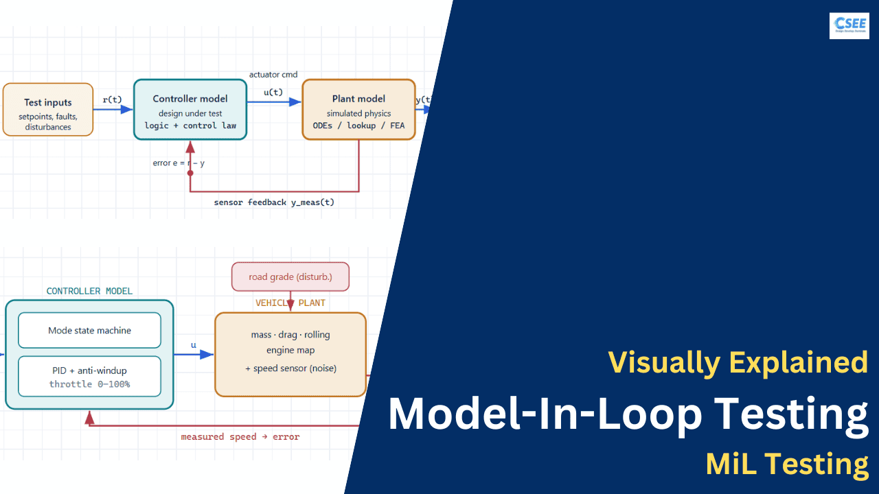
A MiL setup has a small, repeatable anatomy. Once you can name every block and every signal, you can read any MiL model on any project. The heart of it is a loop: the controller decides, the plant reacts, sensors report, and the controller decides again. Surrounding that loop is a test harness that stimulates it and judges the result.
The building blocks
- Reference / setpoint r(t)
- What we want the system to do — the target speed, target temperature, desired position. Supplied by the test harness.
- Controller model
- Reads the error between reference and measured output and computes an actuator command. This is the design under test.
- Actuator command u(t)
- The controller’s decision: throttle percentage, valve opening, motor voltage. It enters the plant.
- Plant model
- Transforms the command into a physical response, producing the true output y(t) — how the system actually moves, heats, or accelerates.
- Sensor / feedback path
- Measures y(t), often adding realistic imperfections: noise, delay, quantization, bias. Returns y_meas(t) to close the loop.
- Test harness
- The scaffolding around the loop: it injects inputs, sequences scenarios, logs signals, and runs pass/fail assessments against requirements. In MiL practice this harness is kept separate from the controller model so the controller stays pristine and reusable in later stages.
Keeping test stimulus and assessment outside the controller model is a discipline that pays off enormously. The exact same controller model can then be reused unchanged for SiL and PiL, and the exact same harness can be pointed at the model, the code, or the target. This is what makes back-to-back equivalence testing possible — identical inputs, identical checks, only the block under test swapped.
Everything downstream depends on the quality of two models: the controller and the plant. The controller is the thing you are designing, so its correctness is the goal. The plant, by contrast, is a means to an end — but a MiL result is only as trustworthy as the plant that produced it. We examine each in turn.
06 / PLANT
Plant modeling in depth
A plant model is a mathematical stand-in for the physical world the controller will command. It is arguably the most underappreciated part of MiL: teams pour attention into the controller and treat the plant as an afterthought, then wonder why their beautifully verified controller misbehaves on real hardware. MiL results inherit the fidelity of the plant. Garbage plant, garbage confidence.
Ways to build a plant model
Plant models span a spectrum from purely theoretical to purely measured, and real projects usually blend approaches.
| Approach | How it’s built | Strengths | Weaknesses |
|---|---|---|---|
| First-principles (white box) | Physics equations: Newton’s laws, thermodynamics, circuit theory, expressed as differential equations. | Transparent, extrapolates well, no test data needed. | Hard for complex or poorly understood systems; parameters may be unknown. |
| Data-driven (black box) | System identification from measured input/output data; fits a transfer function or neural model. | Captures real behavior including quirks; fast to obtain if data exists. | Needs hardware/data up front; poor extrapolation outside tested range. |
| Grey box | Physics structure with parameters tuned to measured data. | Best of both: physical insight plus empirical accuracy. | Requires both modeling skill and data. |
| Lookup / map based | Tabulated measured responses (e.g. engine torque maps) interpolated at runtime. | Fast to simulate, faithful to measured points. | Interpolation error between points; large memory. |
| Multi-domain (physical networks) | Acausal component libraries (electrical, mechanical, hydraulic, thermal) assembled like a schematic. | Handles coupled domains naturally; reusable components. | Can be computationally heavy; solver stiffness. |
Fidelity: matching the plant to the question
A crucial skill is choosing the right level of plant fidelity for the test at hand. A high-fidelity plant that models every nonlinearity is not automatically better — it is slower, harder to build, and can obscure the behavior you are trying to study. Engineers typically maintain more than one plant model:
- A low-fidelity / reduced-order plant for fast, early control-law development and broad scenario sweeps. It runs quickly, so you can test thousands of cases.
- A high-fidelity plant for final MiL verification, capturing nonlinearities, saturation, friction, thermal effects, and sensor imperfections that determine whether the design truly holds up.
Add plant detail only until the controller’s decisions stop changing. If including a nonlinearity does not alter which control action is chosen or whether a requirement passes, that detail is buying simulation time without buying confidence. The right plant is the simplest one that still exposes the failure modes you care about.
What a good plant model represents
Beyond nominal physics, a MiL-grade plant often includes elements that make the loop realistic enough to trust: actuator dynamics and saturation limits (a valve cannot open past 100%), sensor noise and bias, transport and computation delays, quantization from analog-to-digital conversion, and — critically — fault injection hooks so you can simulate a stuck sensor, a broken actuator, or an out-of-range input. Fault handling is frequently where the most important requirements live, and the plant is where those faults are introduced.
With the plant understood as the simulated world, we turn to the star of the show: the controller model, which is the artifact MiL is ultimately designed to prove correct.
07 / CONTROLLER
Controller modeling in depth
The controller model is the design under test — the executable specification of the algorithm you are building. In model-based design it is typically expressed as some combination of continuous/discrete block diagrams for the control mathematics and state machines for the mode and supervisory logic.
Two languages inside one controller
Most real controllers are a marriage of two modeling styles, because real control problems have two natures:
- Data-flow / block diagrams express continuous computation: sums, gains, integrators, filters, PID laws, coordinate transforms. Signals flow left to right through blocks. This is ideal for the “how much” of control — how much throttle, how much current.
- State machines / statecharts express modal and event-driven logic: startup, running, fault, shutdown; “if temperature exceeds limit, enter derate mode.” This is ideal for the “what mode are we in” of control — the discrete decisions and transitions.
A cruise controller, for example, uses a state machine to decide whether it is OFF, STANDBY, ACTIVE, or OVERRIDE, and a block diagram to compute the throttle command whenever it is ACTIVE. MiL must exercise both: every state transition and the numerical control law in each state.
Fixed-point and code-readiness concerns
Because the controller model is destined to become embedded code, MiL is also where implementation-facing decisions get validated at the model level. Two stand out:
- Data types & fixed-point scaling
- Many embedded targets lack fast floating-point units, so controllers are implemented in fixed-point arithmetic. Engineers model the chosen word lengths and scaling and run MiL to confirm the design still meets requirements despite quantization and overflow risk. Catching a fixed-point overflow in MiL is trivial; catching it in the field is a recall.
- Discrete sample time
- The controller will run on a periodic schedule (say every 10 ms). The MiL model uses that discrete sample time so the simulated behavior reflects how the real, sampled controller will actually compute — not an idealized continuous version.
- Modeling standards & guidelines
- To keep a model code-generatable and readable, teams enforce modeling guidelines (naming, block usage, complexity limits). Adhering to these in the controller model is what lets MiL confidence flow cleanly into SiL.
The controller model verified in MiL must be the same model from which code is later generated. If a team maintains one “nice” model for MiL and a separate hand-tweaked model for code generation, the MiL results no longer say anything trustworthy about the shipped software. Single-source the controller model; that is the entire bargain of model-based design.
Now that we can name the controller, the plant, and the harness, we can look at the two fundamental ways of wiring them together for a test: open-loop and closed-loop.
Advertisement
08 / TEST TOPOLOGY
Open-loop vs closed-loop MiL
There are two fundamental topologies for a MiL test, and choosing between them is one of the first decisions in designing any test case. In open-loop testing you feed the controller pre-recorded inputs and check its outputs directly. In closed-loop testing you wire the controller to a live plant so its outputs feed back and influence its next inputs.
When to use each
Open-loop MiL is ideal for deterministic verification of specific logic. Because there is no feedback, the controller’s output for a given input is fixed and repeatable, which makes it perfect for checking exact requirement conformance (“when input is this, output must be that”), for driving coverage of every branch in a state machine, and for regression testing where you compare today’s output against a saved baseline. It is also the natural form for back-to-back testing, since you can replay identical recorded inputs into the model and into the generated code.
Closed-loop MiL is essential for anything about dynamics and stability. Only with the plant in the loop can you observe whether the controller keeps the system stable, how fast it settles, whether it overshoots, how it rejects disturbances, and whether the combined system meets performance requirements. Closed-loop tests reveal emergent behavior that open-loop testing simply cannot — oscillation, limit cycles, windup — because those arise from the interaction between controller and plant.
| Dimension | Open-loop | Closed-loop |
|---|---|---|
| Feedback | None | Plant output returns to controller |
| Best for | Logic, requirement conformance, coverage, regression | Stability, performance, dynamics, disturbance rejection |
| Determinism | Fully deterministic; easy exact checks | Emergent; checks are usually tolerance-based |
| Plant needed? | Not required | Required (and its fidelity matters) |
| Typical assessment | Output equals expected value | Signal stays within bounds / envelope |
Mature MiL suites use both: open-loop tests to pin down every logical requirement and drive coverage, and closed-loop tests to prove the controller actually controls. With topology understood, we can lay out the full workflow that ties it all together.
09 / WORKFLOW
The end-to-end MiL workflow
MiL is not a single button press; it is a repeatable sequence that turns requirements into evidence. The steps below are genuinely sequential — each depends on the one before — which is why numbering them is meaningful rather than decorative.
Step by step
- Capture and link requirements. Every requirement the controller must satisfy is written down and, ideally, linked to the model elements that implement it and the tests that verify it. This traceability is the backbone of the whole effort and is mandatory under safety standards.
- Build the controller and plant models. Develop the controller (the design under test) and a plant of appropriate fidelity. Early on both may be rough; they mature together.
- Create the test harness and cases. Wrap the controller in a harness that supplies inputs and evaluates outputs. Derive test cases directly from requirements — each requirement should map to at least one test.
- Simulate and assess. Run the scenarios. Automated assessments (assertions, verification blocks, tolerance checks) decide pass or fail rather than an engineer eyeballing plots.
- Measure coverage. Instrument the model to see which parts were actually exercised. Uncovered logic is untested logic, no matter how many cases you ran.
- Debug and refine. Failures and coverage gaps drive changes — to the controller (a real bug), the plant (unrealistic assumptions), or the tests (missing cases). Then re-run.
- Report and sign off. When requirements pass and coverage targets are met, generate a report as evidence and hand the verified model to the next stage, SiL.
The reason MiL scales to thousands of test cases is that steps 4–7 are automated. Test suites run unattended (often overnight or on every commit in continuous integration), assessments decide pass/fail without human judgment, coverage is collected automatically, and reports are generated on completion. Manual MiL is possible; automated MiL is what makes it industrial.
Advertisement
10 / TEST DESIGN
Requirements-based test design
The credibility of MiL rests on a simple principle: tests come from requirements, not from the model. If you write tests by looking at what the model does, you will only confirm that the model does what it does — a tautology. Tests derived independently from requirements ask the sharper question: does the model do what it was supposed to do?
From requirement to test case
A well-formed MiL test case has four parts, and every requirement should produce at least one:
- Preconditions / setup
- The initial state and configuration: initial speed 0, mode OFF, plant parameters nominal.
- Stimulus / inputs
- The time-varying signals applied: driver presses SET at t=2s, road grade increases at t=5s.
- Expected behavior
- What the requirement says must happen: vehicle reaches target speed within 8s and stays within ±1 km/h.
- Pass/fail assessment
- The automated check that decides the verdict: an assertion on settling time and steady-state error.
Categories of test cases every MiL suite needs
- Nominal cases confirm the controller does the right thing under normal conditions — the happy path.
- Boundary cases push inputs to the edges of their valid ranges, where off-by-one and saturation bugs hide.
- Robustness cases add noise, delay, and parameter variation to confirm the design tolerates the real world’s imperfection.
- Fault cases inject failures — a stuck sensor, an out-of-range signal, a lost actuator — and verify the controller detects and reacts correctly. These often carry the most safety weight.
- Regression cases re-run previously passing scenarios to ensure new changes did not break old behavior.
Requirements-based tests prove the model does what it should. Coverage analysis then reveals whether any model behavior was never exercised by those tests. Together they close the loop: requirements-based testing checks intended behavior, coverage exposes unintended or untested behavior. Neither alone is sufficient, which is why the next section on coverage is inseparable from this one.
11 / COVERAGE
Coverage metrics and what they mean
Coverage answers a haunting question: “we ran a lot of tests — but did we actually exercise all of the model?” A model can pass every requirements-based test while entire branches of its logic never once execute. Coverage instruments the model during simulation and records which structural elements were reached, giving an objective, measurable gauge of test completeness.
The coverage ladder
Structural coverage metrics form a hierarchy of increasing strictness. Higher metrics subsume lower ones — achieving a stronger metric implies the weaker ones are also met.
| Metric | What it requires | Example |
|---|---|---|
| Execution / statement | Every block or statement runs at least once. | Each block in the model was reached. |
| Decision (branch) | Every decision takes both true and false outcomes. | An if is tested both when it holds and when it doesn’t. |
| Condition | Every boolean sub-condition takes both values. | In A && B, A and B are each tested true and false. |
| MC/DC | Each condition independently shown to affect the decision outcome. | Prove A alone flips the result, and B alone flips it. |
| Lookup-table / boundary | Table breakpoints and interpolation intervals are exercised. | Inputs hit each region of a map, including edges. |
| Signal range | Signals span their expected min/max during testing. | Speed signal actually reached both 0 and top value. |
MC/DC — the safety-critical standard
Modified Condition/Decision Coverage (MC/DC) deserves special attention because safety standards for aviation and automotive frequently demand it for the most critical software. Decision coverage alone can be fooled: with the expression A && B, testing (true,true) and (false,false) achieves full decision coverage while never proving that B matters. MC/DC closes this by requiring that each condition be shown, holding others fixed, to independently change the decision’s outcome. It is the strictest practical structural metric and is the reason MiL suites for safety functions are so thorough.
Reading coverage results honestly
Coverage is a powerful tool that is easily misused. Three cautions:
- 100% coverage is not proof of correctness. It proves every element ran, not that every element is right. A test can execute a block and still pass despite that block being wrong, if the assessment is weak. Coverage measures test thoroughness, not test quality.
- Gaps are diagnostic, not just a grade. An uncovered branch is a question: is there a missing test case, or is that branch dead code that can never execute? Both answers matter — the first drives new tests, the second drives model simplification.
- Achieve coverage with requirements-based tests first. If requirements-based tests leave gaps, that may signal missing requirements. Only after that should you add tests specifically to close remaining structural gaps — and each such test should still be justified.
Some toolchains can automatically generate test inputs that drive a model to full coverage, and can even prove that certain conditions are unreachable (dead logic) or that an assertion can never be violated. Used alongside requirements-based testing, this turns coverage-closing from manual guesswork into an analytical activity.
Advertisement
12 / NUMERICS
Solvers, time steps, and signals
A MiL simulation is ultimately a numerical computation marching forward in time. The choices about how time advances and how signals are represented have real consequences for both accuracy and the validity of later stages, so they deserve explicit understanding rather than acceptance of defaults.
Fixed-step vs variable-step solvers
A solver advances the simulation from one instant to the next. There are two families:
- Variable-step solvers
- Automatically shrink the time step when signals change rapidly and grow it when things are calm, delivering accuracy efficiently. Excellent for early design exploration and for continuous plant models. But their non-uniform timing does not resemble how a real, periodically-sampled controller runs.
- Fixed-step solvers
- Advance by a constant increment every step. This mirrors the periodic execution of an embedded controller, which is exactly why the controller portion of a MiL model is run at a fixed, discrete sample time. Fixed-step is also required for real-time execution later in HiL.
A common and pragmatic arrangement is a mixed simulation: the continuous plant may use a variable- or small fixed-step continuous solver, while the discrete controller runs at its true sample time. This reflects physical reality — the world is continuous, the controller is sampled — and keeps MiL representative of the eventual implementation.
Continuous, discrete, and sampled signals
Signals in a MiL model carry an implicit contract about when they hold meaningful values. Continuous signals are defined at every instant; discrete signals update only at sample instants and hold their value in between (zero-order hold). Getting this right matters because a controller that reads a continuous plant output must sample it, and modeling that sampling — along with the accompanying quantization and delay — is what makes MiL predict real behavior rather than an idealized one.
Too large a step can miss fast dynamics entirely, making an unstable design look stable; too small wastes enormous time. A design that only passes with a suspiciously fine step is a warning sign that the model or the solver configuration — not the controller — is carrying the result. Always confirm results are stable with respect to reasonable solver changes.
13 / EQUIVALENCE
Back-to-back and equivalence testing
One of the most valuable things MiL enables happens at the seam between stages. Because the controller model and the code generated from it are supposed to be equivalent, you can run the same test vectors through both and compare outputs numerically. This is back-to-back testing, and it is the mechanism that lets MiL confidence flow safely into SiL and PiL.
The logic is elegant. If MiL has proven the model correct against requirements, and back-to-back testing proves the generated code produces the same outputs as the model within tolerance, then the code inherits the model’s verified correctness for those scenarios. You do not have to re-verify the algorithm from scratch at the code level; you only have to verify equivalence. This dramatically reduces the verification burden of the later stages — and it is only possible because MiL established a trusted baseline first.
Equivalence checks are almost always tolerance-based rather than bit-exact, because model simulation and compiled code can differ slightly in floating-point rounding, and fixed-point implementations deliberately quantize. The engineer defines acceptable tolerances per signal; a difference within tolerance passes, a larger one flags a genuine discrepancy to investigate — often a fixed-point scaling problem, an unintended data-type cast, or a solver mismatch.
MiL (model meets requirements) → back-to-back MiL/SiL (code matches model) → back-to-back SiL/PiL (target matches host) → HiL (system matches simulation). Each link is a comparison, and each comparison is cheap relative to re-proving correctness. This chain is why model-based design can certify complex software efficiently — and MiL forges its first link.
14 / TOOLS
The tools ecosystem
MiL is a practice, not a product, and several toolchains support it. By far the most common in industry is the MATLAB/Simulink family, but the concepts transfer across environments. What follows describes the categories of tooling any MiL workflow needs, with representative examples, so you can recognize the equivalents in whatever environment you use.
The modeling environment
At the center is a graphical modeling and simulation environment where controller and plant models are built and run. Simulink (with Stateflow for state machines) is the dominant example; it provides the block libraries, the solvers, and the simulation engine. Comparable environments exist — Ansys SCADE (strong in avionics), ETAS ASCET, and various open modeling languages such as Modelica (implemented by tools like Dymola, OpenModelica, and Simulink’s own physical-modeling add-ons) for acausal multi-domain plant modeling.
Test authoring and management
On top of the modeling environment sit tools to author, organize, and run test cases and to assess results automatically — for example Simulink Test, which manages test harnesses, test sequences, and assessments. Dedicated automotive test frameworks such as dSPACE‘s tooling and Vector‘s CANoe/vTESTstudio play in adjacent and later stages.
Coverage and verification analysis
Coverage collection (execution, decision, condition, MC/DC) comes from tools like Simulink Coverage. Formal analysis — automatic test generation, dead-logic detection, and property proving — comes from tools like Simulink Design Verifier (built on formal methods). Modeling-standard checking (guideline compliance) comes from tools like the Model Advisor and Simulink Check.
Code generation (for the stages after MiL)
Although code generation belongs to SiL onward, it is part of the same ecosystem and matters to MiL because the controller model must be code-generatable. Embedded Coder generates production C/C++; HDL Coder targets FPGAs; TargetLink from dSPACE is a widely used production code generator in automotive.
Requirements and traceability
Requirements management and linking — connecting each requirement to model elements and tests — is handled by tools like Simulink Requirements, often integrated with enterprise requirement databases such as IBM DOORS or Polarion.
| Category | Job in MiL | Representative tools |
|---|---|---|
| Modeling & simulation | Build and run controller + plant models | Simulink / Stateflow, SCADE, ASCET, Modelica tools |
| Physical plant modeling | Multi-domain acausal plant models | Simscape, Modelica/Dymola, GT-SUITE, AMESim |
| Test authoring & run | Harnesses, sequences, assessments | Simulink Test, vTESTstudio, dSPACE tooling |
| Coverage | Structural coverage incl. MC/DC | Simulink Coverage, VectorCAST |
| Formal analysis | Auto test-gen, dead logic, property proof | Simulink Design Verifier, Polyspace, SCADE Prover |
| Standards checking | Modeling-guideline compliance | Model Advisor, Simulink Check |
| Code generation | Model → production code (later stages) | Embedded Coder, TargetLink, HDL Coder |
| Requirements & trace | Link requirements ↔ model ↔ tests | Simulink Requirements, IBM DOORS, Polarion |
Whichever toolchain a team adopts, the anatomy is identical: a modeling environment, a way to author requirement-linked tests, an assessment mechanism, a coverage collector, and a reporting/traceability layer. Learn the roles and you can walk into any MiL setup and know what you are looking at.
15 / WORKED EXAMPLE
A worked example: cruise control
Nothing anchors the theory like a concrete case. Consider a classic automotive controller: adaptive-free cruise control that holds a driver-set speed. We will walk it through the MiL lens — requirements, models, tests, and what MiL catches — using it to make every earlier concept tangible.
The requirements (abbreviated)
- R1 — Activation
- When the driver presses SET above 40 km/h, the system shall capture current speed as the target and enter ACTIVE mode.
- R2 — Regulation
- In ACTIVE mode, the system shall hold vehicle speed within ±1 km/h of target on grades up to 6%.
- R3 — Settling
- After a target change, speed shall settle within ±1 km/h in no more than 10 seconds without exceeding target by more than 2 km/h.
- R4 — Override & disengage
- Pressing the brake shall immediately exit ACTIVE mode; the system shall not command throttle in any non-ACTIVE mode.
- R5 — Actuator limits
- Commanded throttle shall remain within 0–100% and shall not wind up during sustained saturation.
The models
The controller model combines a Stateflow state machine for mode logic (OFF → STANDBY → ACTIVE → OVERRIDE) with a Simulink PID block computing throttle from speed error, including anti-windup for R5. The plant model is a longitudinal vehicle: mass, aerodynamic drag, rolling resistance, road grade as a disturbance input, and an engine map translating throttle to force. Sensor blocks add speed-measurement noise and a small delay.
The tests and what MiL catches
Each requirement becomes one or more test cases, mixing open- and closed-loop:
- R1 → open-loop state-machine tests: press SET at 30 km/h (must stay STANDBY) and at 60 km/h (must go ACTIVE). Drives decision coverage of the activation guard.
- R2 → closed-loop tests holding a target while stepping grade from 0% to 6%. Assessment checks speed stays within ±1 km/h — only observable with the plant in the loop.
- R3 → closed-loop step of target from 60 to 80 km/h; assessment checks settling time and overshoot. This is where a badly tuned PID reveals itself.
- R4 → fault/override tests: apply brake mid-ACTIVE and assert throttle immediately goes to zero and mode leaves ACTIVE. A safety-critical behavior.
- R5 → a sustained steep-grade test that saturates throttle, checking the integrator does not wind up and cause overshoot when the grade eases — a classic bug MiL exposes cheaply.
Without touching a vehicle, a dynamometer, or an ECU, the team proved mode logic, regulation accuracy, transient performance, safety override, and actuator robustness — and measured coverage to confirm nothing was left untested. Every one of these bugs, found here, would have been far more expensive to find on the road. That is MiL earning its place.
Advertisement
16 / SCALE
Running MiL at scale: automation and CI
A handful of tests run by hand is a demonstration; thousands of tests run automatically on every change is an engineering capability. The reason MiL transforms product quality is that it is industrialized — folded into the same continuous-integration machinery that modern software teams use. Understanding how MiL scales explains why it can realistically verify systems with hundreds of requirements and tens of thousands of scenarios.
Continuous integration for models
In a mature workflow, the controller model, plant models, test harnesses, and requirement links all live under version control alongside code. Whenever an engineer commits a change to the model, an automated pipeline springs into action: it checks out the model, runs modeling-guideline checks, executes the full MiL test suite, collects coverage, compares results against saved baselines, and publishes a report — all without human involvement. If a test that used to pass now fails, the pipeline flags the exact commit responsible. This is continuous verification, and it catches regressions within minutes of their introduction rather than months later during integration.
Because the model is the design in model-based development, it must be versioned, diffed, merged, and reviewed with the same rigor as source code. Specialized model-comparison and model-merge tools make graphical models behave sensibly under version control, so that “what changed between these two versions of the controller?” has a precise, reviewable answer.
Parameterized and combinatorial testing
Real controllers must work across ranges of conditions, not single points. MiL scales to this through parameterized tests, where one test template is run across a sweep of parameter values — vehicle mass from empty to fully loaded, road grade from level to steep, ambient temperature across a season, sensor noise across plausible amplitudes. A single test definition can expand into hundreds of concrete runs. Because MiL runs faster than real time and parallelizes across CPU cores and build servers, sweeping a large parameter space overnight is routine. This is something that is simply impossible with physical testing, where each condition would require setting up real hardware.
Baselines, regression, and result management
As a project matures, many tests transition from “does this meet the requirement?” to “does this still behave exactly as it did before?” These baseline (regression) tests store a known-good output and compare every future run against it within tolerance. They are the safety net that lets teams refactor and improve a model confidently: if a change unexpectedly alters behavior anywhere, a baseline test fails and points at it. Managing the volume of results — which tests passed, which failed, coverage trends over time, requirement-verification status — becomes its own discipline, supported by dashboards that turn thousands of individual verdicts into an at-a-glance picture of design health.
| Dimension | Manual MiL | Automated / CI MiL |
|---|---|---|
| Trigger | Engineer runs a test by hand | Every commit / nightly schedule |
| Scale | Tens of cases | Thousands, swept across parameters |
| Verdict | Engineer inspects plots | Automated assessments decide pass/fail |
| Regression catch | Often missed until integration | Caught within minutes, tied to a commit |
| Evidence | Ad hoc notes | Auto-generated, traceable reports |
| Coverage | Rarely tracked | Collected and trended automatically |
The shift from manual to automated MiL is the same shift that transformed software engineering with continuous integration — and it is precisely because the design is a model that this automation is possible. The next question is how those automated verdicts are actually reached, which brings us to assessment techniques.
17 / ASSESSMENT
Judging results: assertions, tolerances, and temporal checks
A test is only as trustworthy as its verdict. The mechanism that turns a simulation run into a definitive pass or fail is the assessment, and MiL offers a spectrum of assessment techniques ranging from simple value checks to expressive temporal specifications. Choosing the right one for each requirement is a craft that determines whether your suite catches real problems or waves them through.
Point and threshold assertions
The simplest assessments check a signal against a fixed condition: “throttle command shall never exceed 100%,” “mode shall equal ACTIVE by t=3s.” These assertions fire the instant they are violated, immediately failing the test and pinpointing the moment of failure. They are ideal for invariants — properties that must hold at all times, such as actuator limits or forbidden states.
Tolerance bands and envelopes
Closed-loop behavior is rarely exact, so many assessments compare a signal against a tolerance band or a time-varying envelope rather than a single value. A settling requirement, for instance, is checked by verifying the speed signal enters and stays within a ±1 km/h corridor around the target after a deadline. Envelope checks are the natural way to express performance requirements, because they capture “close enough” without demanding an unrealistic exact match. They are also how back-to-back equivalence is judged: the code output must stay within tolerance of the model output.
Temporal and sequential assessments
The most expressive requirements describe sequences of events over time: “if a fault is detected, then within 200 ms the system shall enter safe mode and remain there until reset.” Checking this needs an assessment that understands ordering and timing, not just instantaneous values. Temporal assessments — sometimes expressed in a temporal logic or a structured “when/then/within” form — let engineers state these directly and have them evaluated automatically over the whole simulation trace. This is where MiL assessment becomes genuinely powerful, because a great many safety requirements are inherently temporal.
- Assertion
- An always-true invariant; fails the instant it is violated. Best for limits and forbidden states.
- Tolerance / envelope check
- Signal must stay within a band, possibly time-varying. Best for performance and equivalence.
- Temporal assessment
- A timed, ordered relationship between events (when…then…within…until). Best for reactive and safety requirements.
- Baseline comparison
- Output compared against a stored known-good trace within tolerance. Best for regression.
A test with a vacuous or overly lenient assessment does something insidious: it looks like coverage of a requirement while actually verifying nothing, giving false confidence. When reviewing a MiL suite, scrutinize the assessments at least as hard as the inputs. The question is never merely “did we exercise this behavior?” but “would this check actually fail if the behavior were wrong?”
With rigorous assessments feeding an automated pipeline, MiL becomes a dependable verdict machine. To finish rounding out the picture, it helps to place MiL among its close relatives and to see how it looks across different industries.
Advertisement
18 / CONTEXT
Rapid prototyping and MiL across industries
MiL has a sibling that is easy to confuse with it, and it wears slightly different clothes in different industries. Clearing up both makes the whole landscape legible.
MiL vs Rapid Control Prototyping
Rapid Control Prototyping (RCP) is often discussed alongside XiL, and newcomers mix it up with MiL. The distinction is clean once seen: in MiL, both controller and plant are simulated on the host, testing the design. In RCP, the controller runs in real time on powerful prototyping hardware and is connected to the real physical plant, letting engineers try a control strategy on actual hardware early — before committing to a production ECU. RCP is, in a sense, the mirror image of HiL: HiL puts a real controller against a simulated plant, while RCP puts a prototype controller against a real plant.
| Method | Controller | Plant | Purpose |
|---|---|---|---|
| MiL | Model (host) | Model (host) | Verify the control design |
| SiL | Code (host) | Model (host) | Verify the generated code |
| RCP | Prototype real-time HW | Real physical plant | Try control on real hardware early |
| HiL | Real production ECU | Real-time model | Validate integrated system |
How MiL looks in different industries
The core method is universal, but its emphasis shifts with the domain’s risks and regulations.
- Automotive. The birthplace of mass-market MBD. MiL is deeply embedded in the ISO 26262 workflow, with heavy use of back-to-back testing against production code generators and large parameterized suites for powertrain, chassis, and ADAS functions. Plant models range from simple vehicle dynamics to detailed engine and battery models.
- Aerospace. Governed by DO-178C and its model-based supplement DO-331, avionics MiL is exceptionally rigorous, with MC/DC coverage mandatory for the highest assurance level and formal methods used widely. Flight-control laws are verified in MiL against high-fidelity aircraft dynamics models long before flight test.
- Industrial & energy. Under IEC 61508 and its sector standards, MiL verifies controllers for turbines, grids, robotics, and process plants — domains where physical testing is slow, expensive, or hazardous, making simulation especially valuable.
- Medical devices. Increasingly model-based, with MiL supporting the verification and traceability that device regulators expect for software that controls therapy delivery or monitors patients.
Whether you are tuning a flight-control law, a battery thermal manager, a turbine governor, or an infusion pump, the shape is the same: a controller model, a plant model, a requirement-linked test harness, automated assessments, and coverage. The industry changes the fidelity, the standards, and the stakes — not the fundamentals you have learned here.
19 / TRADE-OFFS
Advantages, limits, and pitfalls
MiL is powerful but not magic. Using it well means knowing precisely what it gives you, what it cannot give you, and the failure modes that quietly erode its value. Honest engineering respects all three.
What MiL gives you
Early defect detection
Design errors surface when they are cheapest to fix — before code, hardware, or integration exist.
Faster-than-real-time testing
Freed from real-time constraints, MiL can run many scenarios far faster than the events would take in reality, enabling massive test sweeps.
Safe exploration of danger
Faults, extreme conditions, and destructive scenarios that are unsafe or impossible on real hardware are trivial and repeatable in simulation.
Perfect observability
Every internal signal is visible and loggable. Debugging is far easier than on hardware, where probing is limited.
Reproducibility
A simulated test is deterministic and repeatable to the bit (given fixed settings), so regressions are reliable and results are auditable.
Low cost & parallelism
No rig, no target, no vehicle. Tests scale across CPU cores and CI servers rather than scarce lab hardware.
What MiL cannot give you
MiL’s boundaries are exactly the things it abstracts away. It cannot validate the generated code (that is SiL), the target processor’s behavior (PiL), or the hardware, I/O, drivers, and timing of the real system (HiL). It cannot expose problems the plant model does not represent — if your plant omits a resonance, MiL will never see the controller excite it. And it says nothing about electrical integration, wiring faults, or electromagnetic effects. MiL proves the design; the later stages prove the realization. Treating a passed MiL as full validation is the single most dangerous misunderstanding in the field.
Common pitfalls
- Over-trusting a low-fidelity plant. A controller that looks perfect against an oversimplified plant can fail on real hardware. Match plant fidelity to the risk.
- Testing the model instead of the requirements. Writing tests by observing the model confirms only that the model does what it does. Derive tests from requirements.
- Chasing 100% coverage as a goal in itself. Coverage measures thoroughness, not correctness; padding tests to hit a number without strong assessments is theater.
- Weak assessments. A test that runs but does not truly check the requirement passes vacuously. The pass/fail logic must be as rigorous as the requirement.
- Divergent models. Maintaining a separate “test” model and “production” model breaks the chain of trust into later stages.
- Ignoring solver sensitivity. Results that depend on solver settings are results you do not yet understand.
MiL is necessary but not sufficient. It is the first and cheapest quality gate, and skipping it is foolish — but stopping at it is dangerous. Its confidence must be carried forward and complemented by SiL, PiL, and HiL, each closing a gap MiL cannot reach.
20 / STANDARDS
Standards: ISO 26262, DO-178C, IEC 61508
In safety-critical industries, MiL is not just good practice — it is woven into what regulators and standards expect. These standards are why concepts like requirements traceability, MC/DC coverage, and back-to-back testing are non-negotiable rather than nice-to-have. Understanding them explains the rigor described throughout this tutorial.
| Standard | Domain | How MiL fits |
|---|---|---|
| ISO 26262 | Automotive functional safety | Recommends model-based development and back-to-back testing between model and code; MiL provides requirements-based verification and structural coverage evidence keyed to ASIL levels. |
| DO-178C + DO-331 | Civil avionics software | DO-331 (the model-based supplement) explicitly addresses model verification; MC/DC coverage is mandated at the highest design assurance level, and MiL is where model-level evidence is produced. |
| IEC 61508 | General industrial functional safety | The parent functional-safety standard; endorses simulation, structural coverage, and traceable verification that MiL directly supplies for SIL-rated functions. |
| ISO 25119 / EN 50128 | Agricultural machinery / rail | Sector adaptations with similar expectations for model verification, coverage, and traceability that MiL activities satisfy. |
The common thread across all of them is a demand for evidence: evidence that every requirement is tested, that the tests exercise the design thoroughly (measured by coverage, with MC/DC at the top tiers), that the implementation matches the verified design (back-to-back testing), and that all of this is traceable end to end. MiL, executed with the discipline described here, is a primary engine for generating exactly that evidence — which is why it is the default first verification stage in automotive, aerospace, rail, and industrial control development.
Standards grade functions by how catastrophic their failure would be — ASIL A–D in automotive, DAL A–E in avionics, SIL 1–4 in industrial. The higher the level, the stricter the verification: more coverage rigor (up to MC/DC), stronger independence between the people writing requirements and those testing, and more complete traceability. MiL scales its own rigor to match.
Advertisement
21 / FAQ
Frequently asked questions
A few questions come up again and again from engineers and students meeting MiL for the first time. Answering them directly resolves the most common confusions.
Is the plant model part of “the model” in Model-in-the-Loop?
No — and this is the single most common point of confusion. The “Model” in the name refers to the controller being a model. The plant is also modeled, but the letter describes the maturity of the thing under test, not its surroundings. That is why in SiL the controller becomes software and in HiL it becomes hardware, while the plant frequently stays a model throughout.
If MiL passes, is my software verified?
No. MiL verifies the design, not the implementation. It says nothing about whether the generated code matches the model (that is SiL and back-to-back testing), whether the target processor computes the same values (PiL), or whether the wired-up hardware behaves correctly under real timing and I/O (HiL). A passed MiL is a necessary milestone, never a final one.
How much plant fidelity do I actually need?
Exactly enough to expose the failure modes that matter for the test at hand — and no more. A good heuristic: keep adding plant detail only while it continues to change the controller’s decisions or the pass/fail outcome. Once more detail stops altering results, it is buying simulation time without buying confidence. Most teams keep a fast low-fidelity plant for exploration and a high-fidelity plant for sign-off.
Do I need closed-loop tests if my open-loop tests pass?
Usually yes. Open-loop tests are excellent for logic, requirement conformance, and coverage, but they cannot reveal anything that emerges from the controller and plant interacting — stability, overshoot, oscillation, disturbance rejection, integrator windup. Those behaviors only appear when the loop is closed. Mature suites use both topologies deliberately.
Isn’t 100% coverage the goal?
Coverage is a measure of test thoroughness, not correctness. You can reach full coverage with weak assessments that verify nothing meaningful, and you can have excellent tests that leave a little coverage genuinely unreachable (dead logic). Treat coverage gaps as questions to investigate — missing test or dead code — and pursue coverage through requirements-based tests first, closing residual gaps with justified additions.
Why keep the test harness separate from the controller model?
Because separation lets the identical controller model flow unchanged into SiL and PiL, and lets the identical harness be pointed at the model, the generated code, or the target. That reuse is exactly what makes back-to-back equivalence testing — the chain of trust between stages — possible. Baking stimulus and checks into the controller breaks that chain.
Can MiL find timing bugs?
Only the logical ones. MiL models the controller’s discrete sample time, so it captures sampling-related design behavior. But it does not run in real time and does not model the target’s execution time, interrupt latency, or scheduling — those belong to PiL and HiL. If a requirement is about how long the real controller takes to compute, MiL is not the stage that verifies it.
Where does MiL end and the next stage begin?
MiL ends when the controller model meets its requirements and coverage targets against an appropriate plant, with results reported and traceable. At that point the verified model is handed to code generation, and SiL takes over to confirm the code matches the model. The boundary is clean precisely because responsibilities were kept separate: MiL owns “is the design right?”, and everything after owns “is the design built right?”
22 / PRACTICE & REFERENCE
Best practices, glossary, and summary
To close, here is a distilled set of practices that separate effective MiL from box-ticking, followed by a reference glossary and a one-paragraph synthesis of everything above.
Best practices, condensed
- Single-source the controller model. The model you verify in MiL must be the model you generate code from. No parallel copies.
- Derive tests from requirements, then close gaps with coverage. Requirements-based first; structural coverage reveals what is left; justify every added test.
- Keep the harness separate from the controller. This enables reuse in SiL/PiL and makes back-to-back testing straightforward.
- Maintain plant models at more than one fidelity. Fast plant for exploration, high-fidelity plant for sign-off; know which failure modes each can expose.
- Model implementation reality early. Use the true discrete sample time, model fixed-point where relevant, and include sensor/actuator imperfections so MiL predicts real behavior.
- Write strong assessments. A test is only as good as its pass/fail check; make assessments as precise as the requirement they verify.
- Automate everything. Run suites unattended in continuous integration; regenerate coverage and reports on every change.
- Confirm solver-independence. Results should be stable under reasonable solver/step changes; if not, understand why before trusting them.
- Prioritize fault and boundary cases. The happy path rarely hides the dangerous bugs; edges and failures do.
- Preserve traceability. Requirement ↔ model element ↔ test ↔ result, end to end — both for quality and for certification.
Glossary
| Term | Meaning |
|---|---|
| MiL | Model-in-the-Loop: controller model tested against a plant model on the host, before code exists. |
| SiL | Software-in-the-Loop: generated code tested (on host) against a plant model. |
| PiL | Processor-in-the-Loop: generated code run on the real target CPU against a plant model. |
| HiL | Hardware-in-the-Loop: real ECU wired to a real-time plant simulator. |
| MBD | Model-Based Design: development approach with an executable model at the center. |
| Plant | Model of the physical system the controller acts on. |
| Controller | The control algorithm being designed; the design under test in MiL. |
| Test harness | Scaffolding that stimulates the controller and assesses its outputs. |
| Open-loop | Controller tested with fixed inputs, no feedback. |
| Closed-loop | Controller and plant interact; output feeds back to input. |
| MC/DC | Modified Condition/Decision Coverage; strictest common structural metric, required for the most critical software. |
| Back-to-back | Running identical inputs through model and code (or host and target) and comparing outputs. |
| Fixed-step solver | Advances simulation by a constant time increment, mirroring a sampled controller. |
| Anti-windup | Technique preventing an integrator from accumulating error while an actuator is saturated. |
| Traceability | Linked chain from requirement to model to test to result. |
The whole thing in one paragraph
Model-in-the-Loop testing is the earliest verification stage of model-based design, in which a controller model — the algorithm you are building — is co-simulated on a host computer against a plant model that stands in for the physical system, so the design can be proven against its requirements before any code or hardware exists. It sits on the ascending arm of the V-model as the first of the XiL stages (MiL → SiL → PiL → HiL), each of which trades speed for realism while carrying MiL’s confidence forward through back-to-back equivalence testing. A MiL setup wires a controller, a plant, and a sensor feedback path inside a separate test harness that injects requirement-derived scenarios and renders automated pass/fail verdicts, using open-loop tests to nail down logic and coverage and closed-loop tests to prove stability and performance. Its value is measured by requirements conformance and structural coverage (up to MC/DC for safety-critical functions), its results are only as trustworthy as the plant’s fidelity and the assessments’ rigor, and its rightful place is as the cheapest, first, necessary-but-not-sufficient quality gate — indispensable, and always to be completed by the stages that follow.
Find every implementation-independent defect in MiL, where it is cheapest — then let each later stage confirm, not re-discover. That single habit is what makes model-based development fast, safe, and certifiable.