Hardware-in-the-Loop · Test Systems Engineering
Building a HiL Test Bench with the Vector VT System
A complete, diagram-driven engineering tutorial covering the architecture, hardware modules, signal conditioning, real-time plant models, closed-loop algorithms, wiring, configuration, and test automation needed to validate an automotive ECU end to end.
What Hardware-in-the-Loop Really Is
Hardware-in-the-Loop (HiL) testing is a technique for validating an embedded controller by connecting the real, physical electronic control unit (ECU) to a simulated version of everything it would normally control. Instead of installing the ECU in a vehicle and driving it around a proving ground, you place it on a bench and surround it with electronics that imitate the sensors, actuators, loads, and communication partners of the real system. The controller cannot tell the difference. It reads voltages, currents, resistances, PWM signals, and bus messages that behave exactly as they would in the car, and it drives outputs that the bench measures and feeds back into a mathematical model of the vehicle.
The word that matters in the name is loop. The ECU produces an output — say, a command to open a throttle valve — and the bench does not merely record that output. It feeds it into a running simulation of the engine, computes the physical consequence (airflow rises, manifold pressure changes, the crankshaft accelerates), and immediately presents the resulting sensor readings back to the ECU. The controller then reacts to those new readings, producing a new output, and the cycle repeats. This continuous, bidirectional exchange runs many hundreds or thousands of times per second, closing a control loop that spans real silicon and simulated physics.
This is fundamentally different from open-loop stimulation, where you simply play recorded signals at a device and watch what it does. A closed loop lets you test emergent behaviour — the way a controller and its environment mutually influence each other over time. You can drive the simulated vehicle through a highway on-ramp, inject a wheel-speed sensor fault at exactly 80 km/h, and observe how the ABS controller recovers, all without any physical risk and with perfect repeatability.
Why engineers invest in HiL
- Safety. Fault conditions that would be dangerous or destructive in a real vehicle — short circuits, sensor dropouts, brake-line failures — can be injected on the bench in complete safety.
- Repeatability. A test scenario runs identically every time. When a defect appears, it can be reproduced deterministically, which is the single most valuable property when debugging intermittent behaviour.
- Coverage. Rare and extreme operating points — a sensor at the edge of its range, a bus flooded with error frames, an actuator drawing over-current — are trivial to reach in simulation and nearly impossible to provoke on demand in a vehicle.
- Automation and cost. Thousands of regression tests can run overnight, unattended, on hardware that costs a fraction of a prototype vehicle and never needs fuel, a track, or a driver.
Open-loop vs. closed-loop, signal-level vs. power-level
Not every HiL bench is the same. Two orthogonal distinctions shape how a bench is built and what it can prove.
The first is open-loop versus closed-loop. An open-loop bench plays predefined stimuli at the ECU and records its reactions, but the ECU’s outputs do not feed back into a model — the stimulus schedule is fixed in advance. This is adequate for simple I/O checks and some diagnostic testing. A closed-loop bench, the subject of this tutorial, routes the ECU’s outputs through a live plant model whose results become the next stimuli, so the controller and its simulated environment influence each other continuously. Only a closed loop can test the dynamic, emergent behaviour that dominates real-world controller performance — stability, transient response, the interaction of multiple control functions.
The second distinction is signal-level versus power-level HiL. A signal-level bench works with low-power representations of every signal: sensor voltages, PWM waveforms, and bus messages, but the ECU’s power actuator outputs are terminated into small electronic loads rather than driving real hardware. A power-level bench drives genuine high-current loads — real injectors, real motors, real lamps — so the ECU’s power stages experience true inductance, inrush, and thermal behaviour. Power-level HiL is more faithful but more expensive and more constrained; signal-level HiL is more flexible and covers the vast majority of control-logic validation. The VT System spans both: its load modules can present electronic loads for signal-level work or switch in physical loads for power-level fidelity, and the same rack can mix the two per channel according to what each output demands.
The Vector VT System is a modular hardware platform purpose-built to be the electrical interface of exactly this kind of bench. It is the layer of copper, relays, amplifiers, and load electronics that sits between the ECU connector and the simulation software. The rest of this tutorial explains how that layer is architected, how you wire and configure it, what algorithms make the loop close in real time, and how you drive the whole thing from Vector’s CANoe software.
Where HiL Sits in the V-Model
Automotive software is developed along the classic V-model: requirements and design descend the left arm, implementation sits at the bottom, and integration and verification climb the right arm. Testing is not a single stage but a graded series of environments, each replacing more of the simulation with real hardware. Understanding this ladder makes it clear precisely what HiL verifies and what it deliberately does not.
| Stage | Controller under test | Environment | Timing | Primary purpose |
|---|---|---|---|---|
| MiL | Control model (Simulink) | Plant model | Non-real-time | Verify control logic against requirements |
| SiL | Generated C code on PC | Plant model | Non-real-time | Verify code equals model behaviour |
| PiL | Code on target processor / eval board | Plant model | Near-real-time | Verify timing & compiler on real silicon |
| HiL | Complete production ECU | Real I/O + real-time plant | Hard real-time | Verify full electrical & system behaviour |
→ scroll table sideways
The essential leap at the HiL stage is that the object under test is the finished ECU — the same part number that ships in the car, with its production connector, its real microcontroller, its real power supply requirements, and its real diagnostic behaviour. Everything upstream (MiL, SiL, PiL) tests the software in isolation. HiL is the first and only pre-vehicle stage that tests the software together with the hardware it will actually run on, driving real electrical loads and communicating over real bus wires. That is precisely the gap the VT System is engineered to fill.
The VT System at a Glance
The Vector VT System is a modular, rack-based hardware platform for connecting ECUs to a test environment. Rather than being one monolithic box, it is a family of plug-in modules, each specialised for a class of electrical signal, that slot into a common backplane. You assemble exactly the set of modules your ECU requires — a few analog channels here, a bank of load switches there, a bus interface, a programmable power supply — and the backplane wires them all to a shared internal bus and power rail. The result is a compact, serviceable, and reconfigurable test interface that can be re-tasked from one project to the next simply by swapping cards.
Three design ideas define the platform:
Modularity
Function-specific cards (analog, digital, load, bus, power) share one backplane. Build only what the ECU pinout needs.
Integrated fault insertion
Most I/O modules include on-board relays to simulate opens, shorts-to-battery, and shorts-to-ground per channel.
Native CANoe control
Every channel is addressable from CANoe as a symbolic system variable — no separate driver stack to maintain.
The last point is the platform’s defining commercial advantage. The VT System is designed to be operated from within CANoe, Vector’s development and test tool for networked ECUs. The same tool that already simulates the CAN, LIN, FlexRay, and Automotive Ethernet buses in your bench also controls the analog voltages, the load currents, and the fault relays. There is a single configuration, a single set of test sequences, and a single measurement window covering both the network side and the electrical I/O side of the ECU. This tight coupling removes an entire category of integration effort that plagues benches built from mixed-vendor instrumentation.
Physically, the modules are front-connectorised: the ECU wiring harness terminates on the module fronts (typically via D-Sub connectors and breakout boxes), while the rear of each card mates with the backplane. Signal conditioning, measurement amplifiers, load electronics, and the relays for fault insertion all live inside the module. From the test engineer’s perspective, each module presents a clean set of named channels that can be read, driven, switched, and faulted from software.
The backplane and internal synchronisation
The backplane is more than a power-distribution board. It carries a shared communication bus that lets modules exchange data with the controlling host and, critically, a synchronisation signal that keeps every module on a common time base. When the real-time loop commands a new set of outputs, you generally want them to take effect together — a set of correlated sensor values that represent a single, consistent instant of simulated time. The backplane’s timing infrastructure allows modules to latch their outputs coherently and to timestamp their measurements against the same clock, so that the model always sees a self-consistent snapshot of the ECU rather than a smear of values captured at slightly different moments.
This coherence matters more than it first appears. Consider an engine controller that cross-checks crankshaft position against camshaft position to identify which cylinder is firing. If the crank and cam signals were generated from slightly different time references, the ECU could compute an impossible phase relationship and set a plausibility fault — a fault caused entirely by the bench, not the ECU. Synchronised output latching across modules eliminates that class of artefact.
Scalability across multiple racks
A single backplane hosts a fixed number of module slots. Large ECUs — a body controller with hundreds of pins, or a domain controller consolidating many functions — exceed one rack’s capacity. The VT System scales by linking multiple racks so their modules appear as one contiguous channel space to the host, sharing the same synchronisation so that a signal generated in one rack stays time-aligned with a measurement taken in another. From the test engineer’s point of view the physical partitioning is invisible: channels are addressed by name regardless of which rack they physically live in.
System Architecture
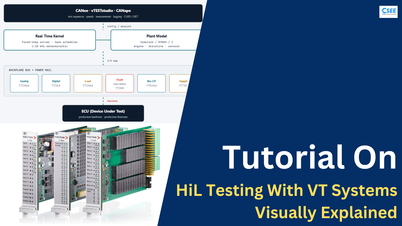
A complete VT-based HiL bench is a stack of cooperating layers. At the top is the test authoring and orchestration software; at the bottom is the ECU’s copper. Between them sit the real-time execution of the plant model and the physical signal conditioning of the VT hardware. The diagram below shows the full closed loop, following a signal from the ECU output, through the VT hardware into the model, and back through the VT hardware to the ECU input.
Layer responsibilities
Each layer has a strict responsibility and a strict timing budget. Keeping these boundaries clean is what makes a HiL bench deterministic and maintainable.
Host / test layer
Runs on a standard Windows PC. This is where the test engineer works: CANoe hosts the configuration, panels, and measurement display; vTESTstudio authors test cases; CANape handles measurement and calibration of internal ECU variables. This layer is soft real-time — it issues commands, collects results, and logs data, but it does not participate in the microsecond-level timing of the control loop.
Real-time layer
A dedicated real-time execution environment — a Vector real-time kernel running on a real-time server PC or a VN8900-class interface — executes the plant model at a fixed, deterministic step rate (commonly 1 kHz to 10 kHz, sometimes higher for power-electronics models). It reads the ECU’s outputs as measured by the VT modules, advances the physics one time step, and writes the resulting stimulus back to the VT modules. Determinism here is non-negotiable; a missed deadline corrupts the physics.
VT System layer
The physical interface. Modules convert between the digital world of the model and the analog electrical world of the ECU: digital-to-analog conversion to generate sensor voltages, analog-to-digital conversion to measure ECU outputs, power electronics to sink actuator currents, and relays to insert faults. Bus interface modules bridge the simulated network into the ECU’s real transceivers.
DUT layer
The ECU itself, powered by a programmable supply (so you can test brown-out, load-dump, and cranking-voltage behaviour) and wired to the VT modules through a breakout box that makes every pin individually accessible for probing and fault insertion.
The Module Catalog
The VT System’s expressiveness comes from its module families. Modules are grouped by the electrical function they perform. The table below summarises the representative families you will assemble a bench from; exact channel counts and current ratings vary by module revision, so always confirm against the current datasheet for your specific hardware.
| Family | Class | Primary function | Typical channels | Fault insertion |
|---|---|---|---|---|
| VT1004A | Load / switch | Switch and load ECU actuator outputs (lamps, valves, relays); high-side & low-side; measure output voltage/current; PWM measurement | 4 | Yes (per channel) |
| VT2004A | Analog | Generate and measure analog voltages; simulate resistive & voltage sensors; measure ECU analog outputs | 4 | Yes |
| VT2516 / VT2816 | Digital / mixed | Measure and stimulate digital and analog signals; frequency & PWM in/out; switch inputs | 16 / mixed | Yes |
| VT2710 | General purpose | FPGA-based module for custom / high-speed signal processing not covered by standard cards | Configurable | App-defined |
| VT2848 | Digital I/O / matrix | High-channel-count switching, error/fault relay matrices, break/short routing | 48 | Matrix |
| VT6104A | Network interface | Bring CAN / CAN FD / LIN / FlexRay bus interfaces into the rack for restbus simulation | Multi-bus | Bus-level |
| VT7001A | Power supply | Programmable ECU supply; ramp, brown-out, load-dump, cranking profiles; current measurement | 1–2 outputs | Supply faults |
| VT8006A | Backplane / rack | Housing + backplane bus + power distribution for the module stack | 6 slots | — |
→ scroll table sideways
Choosing modules from an ECU pinout
Module selection is a mechanical exercise driven by the ECU’s connector pinout. Walk every pin of the ECU connector and classify it, then tally the channels each class needs:
- Analog inputs to the ECU (temperature, pressure, position sensors) → analog generation channels (VT2004A).
- Analog / digital outputs from the ECU (PWM to a solenoid, a status line) → measurement channels or load modules (VT1004A, VT2816).
- Power actuator drives (injectors, motors, lamps) → load modules able to sink the real current (VT1004A).
- Bus pins (CAN-H/CAN-L, LIN, FlexRay) → network interface (VT6104A) plus the restbus simulation in CANoe.
- Supply and ground pins → programmable supply (VT7001A).
Add margin: real projects add channels for spare pins, wake-up lines, and instrumentation. The backplane slot count (e.g. six per VT8006A) determines how many modules you can host; large ECUs use multiple linked racks.
Signal Conditioning Chain
The heart of the VT System’s job is signal conditioning — converting the clean digital numbers the model works in into the messy analog electrical reality the ECU expects, and vice versa. Consider a coolant-temperature sensor. In the real car it is an NTC thermistor whose resistance falls as temperature rises; the ECU applies a bias voltage through a pull-up resistor and reads the divider voltage. To fool the ECU on the bench, the analog module must present the ECU with the same resistance (or the same divider voltage) that a real thermistor at the model’s current temperature would produce.
The stimulus path
Going from model to ECU, three transformations happen in series. First, scaling maps the physical quantity (92.4 °C) through the sensor’s characteristic curve to an electrical target (a resistance, or a divider voltage). Second, the module’s signal generator — a DAC for voltage sources, or a programmable resistance network for resistive sensors — physically realises that target on the output terminal. Third, an optional fault relay can override the clean signal with an open circuit, a short to ground, or a short to battery, to test the ECU’s fault detection.
The response path
Going from ECU to model, the flow reverses. The ECU drives an output — often a PWM waveform to a solenoid or motor. A load module presents the correct electrical load so the ECU’s output stage behaves as it would in the car (an unloaded output can read wrong or trip a diagnostic). The module simultaneously measures the waveform, and a decode step extracts the meaningful quantity — the PWM duty cycle, the switching frequency, the current — which is scaled back into engineering units and handed to the model as the actuator command.
Sensor emulation in detail
Different sensor types demand different emulation strategies, and the analog module has to realise each faithfully enough that the ECU’s front-end circuit is fooled.
- Resistive sensors (NTC/PTC thermistors, potentiometric position sensors) are read by the ECU as part of a resistor divider it powers itself. Emulating them means presenting a programmable resistance, not a voltage — because the ECU’s own pull-up sets the current, and the ECU may also monitor that the total resistance stays within a plausible band. Presenting a voltage instead of a resistance can defeat the ECU’s diagnostic that checks its own reference.
- Ratiometric voltage sensors (many pressure and position sensors) output a voltage that scales with the ECU’s supply. Emulation must track the ECU’s actual reference voltage so the ratio stays correct even if the supply drifts, otherwise the ECU’s ratiometric compensation produces a wrong reading.
- Active / digital sensors (Hall-effect, magneto-resistive speed sensors, SENT and PSI5 sensors) output edges or encoded digital frames rather than analog levels. These are generated by digital or FPGA-based channels that reproduce the exact edge timing, and for protocol sensors the full frame format including its checksum.
- Thermocouples and low-level sensors produce millivolt-scale signals that demand high-resolution generation and careful shielding, because bench noise that would be negligible on a 5 V signal is significant on a 10 mV one.
The breakout box
Between the ECU connector and the module fronts sits a breakout box — a passive panel that brings every ECU pin out to an accessible terminal before routing it onward to the VT modules. It exists for three reasons: it makes every pin probeable with a meter or oscilloscope during commissioning and debugging; it provides a defined, labelled point for manual fault insertion when a fault is outside the module’s built-in matrix; and it decouples the fragile ECU connector from the frequently-rewired module side, so re-tasking the bench for a different ECU means rebuilding cheap harness on the breakout side rather than stressing the ECU connector. A well-built breakout box, meticulously labelled and documented, is one of the highest-leverage investments in a durable bench.
Load Simulation & Fault Insertion
Two capabilities distinguish a HiL bench from a simple signal generator: realistic load simulation and systematic fault insertion. Both are built into the VT System’s load and matrix modules.
Load simulation
Real actuators present real electrical loads. An incandescent lamp is a low resistance that draws a large inrush current when cold. A solenoid is an inductor that resists changes in current and generates a back-EMF spike when switched off. A DC motor’s current depends on its speed and torque. The VT load modules emulate these behaviours so the ECU’s driver stages see the loads they were designed for. Depending on the module, loads are realised as switched resistor banks, active current sinks, or genuine physical loads mounted on the bench and switched in by relays. The choice trades fidelity against flexibility: a physical lamp gives perfect thermal-inrush behaviour but is fixed; an electronic sink is fully programmable but must model inrush and inductance in firmware.
Fault insertion (FIU)
The single most valuable thing a HiL bench does is let you provoke faults safely and repeatably. A Fault Insertion Unit is a matrix of relays wired into each signal line. Under software command it can break the connection between the ECU pin and its signal source (open circuit), tie a pin to the battery rail (short-to-battery), tie it to ground (short-to-ground), or connect two pins together (pin-to-pin short). The VT System integrates this capability directly into its I/O and matrix modules, so no separate FIU rack is required for common faults.
| Fault | Relay action | Simulates | ECU behaviour verified |
|---|---|---|---|
| Open circuit | K1 open | Broken wire, disconnected sensor | Open-load diagnostic, DTC set, limp-home |
| Short to battery | K2 close | Chafed harness against +12V | Over-voltage protection, fault code, output disable |
| Short to ground | K3 close | Chafed harness against chassis | Over-current shutdown, DTC, recovery logic |
| Pin-to-pin short | matrix | Adjacent pins bridged | Plausibility checks, cross-signal detection |
| Intermittent | K1 chatter | Loose connector, vibration | Debounce logic, transient rejection |
→ scroll table sideways
Because every relay is a named software channel, fault campaigns become ordinary automated test cases: a test sequence can walk every sensor pin, apply each fault type in turn, wait for the ECU’s diagnostic to react, and read back the resulting diagnostic trouble code over the bus — all unattended, and all perfectly reproducible.
The Real-Time Plant Model
The VT System is the muscle; the plant model is the brain of the simulated world. It is a set of mathematical equations describing how the physical system responds to the ECU’s commands. For an engine ECU the plant model includes the intake manifold dynamics, combustion torque production, crankshaft inertia, and the transfer functions of every sensor. For a chassis controller it includes vehicle mass, tyre-road friction, and wheel dynamics. The model consumes the ECU’s outputs (as measured by the VT modules) and produces the sensor values the ECU should see next.
Where the model runs
Crucially, the plant model does not run on the host PC’s ordinary operating system, because Windows cannot guarantee that a computation finishes within a fixed deadline. Instead it runs on a real-time execution environment — a dedicated real-time kernel — whose only job is to execute the model at a rigid, unvarying step rate. Vehicle-level models are commonly authored in MATLAB/Simulink or Vector’s DYNA4 vehicle-dynamics toolset, then compiled to C code and deployed onto the real-time target. The VT System’s I/O is mapped to the model’s inputs and outputs so that each real-time step reads fresh measurements and writes fresh stimuli.
Model fidelity vs. step rate
There is a direct trade-off between how detailed the model is and how fast it can step. A coarse mean-value engine model runs comfortably at 1 kHz. A crank-angle-resolved model that captures individual combustion events needs a far higher rate. Power-electronics models (inverters, DC-DC converters) may need tens or hundreds of kHz, which is why some benches offload the fastest dynamics to FPGA-based modules (like the VT2710) that compute those loops in hardware, right next to the I/O, without troubling the CPU-based kernel.
| Domain | Dominant dynamics | Step rate | Where it runs |
|---|---|---|---|
| Vehicle dynamics | Mass, suspension, tyres | 100–1000 Hz | RT CPU kernel |
| Mean-value engine | Manifold, torque, speed | 1 kHz | RT CPU kernel |
| Crank-resolved engine | Per-cylinder combustion | 10–50 kHz | RT CPU / FPGA |
| Electric drive / inverter | PWM switching, currents | >100 kHz | FPGA module |
→ scroll table sideways
What a plant model actually contains
It is worth being concrete about the ingredients of a plant model, because they map directly onto the VT channels. A model has three kinds of content. First, state equations — the differential equations that carry the system’s memory: crankshaft speed, manifold pressure, vehicle velocity, coolant temperature. These are what the integrator advances each step. Second, sensor models — the functions that turn internal states into the signals the ECU reads, including each sensor’s characteristic curve, its dynamic lag, and its noise. A temperature that changes instantly in the state equations should reach the ECU through a sensor model with the real sensor’s thermal time constant, or the ECU sees an unphysically fast transient. Third, actuator models — the functions that turn the ECU’s decoded outputs back into forces and flows acting on the states, capturing the actuator’s own dynamics and limits.
This structure is why the signal-conditioning chain of section 06 has scaling and characteristic blocks on both sides: the plant model deliberately works in clean physical quantities, and the boundary layers translate to and from the messy electrical reality. Keeping that separation strict makes the model portable — the same model can drive a MiL simulation, a SiL run, and a HiL bench, with only the boundary layer changing.
Synchronising the real world with the model’s clock
A subtle challenge is that the ECU runs on its own clock, asynchronous to the model’s step. When the model presents a new sensor value, the ECU samples it whenever its own schedule dictates, and it drives its outputs on its own timeline. The bench must therefore sample the ECU’s outputs and present new stimuli at instants that keep the loop coherent despite this asynchrony. Fast-changing outputs like PWM are measured continuously by the module hardware and summarised (as duty and frequency) into each model step, so the CPU loop never has to chase individual edges. This division of labour — fast, continuous processing in the module; slower, coherent exchange with the CPU model — is the key to a bench that is both fast enough and deterministic.
The Closed Loop
Everything above comes together in a single repeating cycle. The sequence diagram traces one real-time step from the moment the clock ticks to the moment the loop is ready for the next tick. This exact sequence repeats deterministically at the model’s step rate for the entire duration of the test.
The elegance of the loop is that the ECU is a full participant. Between step 5 (the bench presents new sensor values) and step 2 of the next cycle (the bench samples the ECU’s response), the real ECU firmware runs its own control algorithm at its own rate on its own silicon. The bench never simulates the controller — it only simulates the world the controller lives in. That separation is what makes HiL a genuine test of the production software rather than a test of a model of it.
Core Functions of Each Layer
It helps to enumerate the concrete functions the VT System performs, because these are the primitives you invoke from test code. They fall into five groups.
Signal generation
Producing a defined electrical output that the ECU reads as a sensor. This includes fixed DC voltages, arbitrary waveforms, PWM outputs of a set frequency and duty, frequency signals (for crankshaft/wheel-speed emulation), and programmable resistances for resistive sensors. Each generation channel is scaled from an engineering value written by the model.
Measurement
Capturing what the ECU produces: voltage, current, PWM duty cycle, frequency, and edge timing. Measurement channels feed the decode-and-scale step that hands values to the model. High-resolution measurement also supports characterisation — recording exactly how an ECU output stage behaves under different loads.
Load and power switching
Presenting realistic loads to ECU driver stages and switching power actuators on and off. This group also covers the programmable ECU supply: ramping the supply voltage to test brown-out thresholds, injecting load-dump transients, and reproducing the sagging voltage profile of engine cranking.
Fault insertion
Commanding the relay matrix to create opens, shorts, and pin-to-pin bridges on any channel, as described in section 07. Exposed as simple on/off channels per fault per pin.
Bus communication
Bridging the simulated network into the ECU. The network interface module carries the physical CAN/LIN/FlexRay/Ethernet lines, while CANoe runs the restbus simulation — sending all the messages the ECU’s communication partners would send, so the ECU sees a fully populated, correctly timed network even though every other node is virtual.
Generate
DC, PWM, frequency, arbitrary waveforms, programmable R.
Measure
V, I, duty, frequency, edge timing, characterisation.
Load / power
Realistic loads, actuator switching, programmable supply profiles.
Fault
Open, short-to-batt, short-to-gnd, pin-to-pin, intermittent.
Communicate
CAN/CAN FD/LIN/FlexRay/Ethernet restbus simulation.
Orchestrate
Sequence, log, evaluate pass/fail, report — from CANoe.
Algorithms Used
A HiL bench is, at bottom, a collection of algorithms running at different rates. This section presents the important ones in pseudocode. They are simplified for clarity but reflect the real structure of what runs on the bench.
11.1 · The real-time loop scheduler
The master algorithm is the deterministic scheduler that drives every step. It uses a hardware timer to release the task at a fixed period and monitors for overruns.
# Fixed-step deterministic HiL loop
const DT = 0.001            # 1 ms step  (1 kHz)
state = initial_state()

while running:
    wait_for_timer_tick()      # blocks until next 1 ms boundary
    t_start = now()

    inputs  = read_vt_inputs()   # sample & decode ECU outputs
    u        = scale_to_engineering(inputs)

    state   = integrate(state, u, DT)   # advance physics one step
    y        = outputs_of(state)          # sensor values for ECU

    stim    = scale_to_electrical(y)
    write_vt_outputs(stim)      # drive DAC / load / R-sim

    log(t_start, u, state, y)

    if now() - t_start > DT:      # deadline missed?
        flag_overrun()            # test result is now invalid
11.2 · Plant integration — fixed-step Runge–Kutta (RK4)
The integrate() call advances the model’s ordinary differential equations by one step. HiL uses fixed-step solvers only — variable-step solvers can’t guarantee a bounded compute time. RK4 is the workhorse: it evaluates the derivative four times per step for good accuracy at modest cost.
# Classic 4th-order Runge-Kutta, fixed step h
function integrate(x, u, h):
    k1 = f(x,            u)
    k2 = f(x + h/2*k1,  u)
    k3 = f(x + h/2*k2,  u)
    k4 = f(x + h*k3,    u)
    return x + (h/6)*(k1 + 2*k2 + 2*k3 + k4)
Here f(x,u) is the plant’s derivative function — the equations of motion. For a single rotating inertia driven by engine torque Te and load torque Tl, for example, f returns angular acceleration (Te − Tl) / J. Simpler models sometimes use forward-Euler (a single derivative evaluation) when the dynamics are slow relative to the step; RK4 is preferred when accuracy at a given step size matters.
11.3 · PWM duty-cycle measurement
Many ECU outputs are PWM. To feed the model an actuator command, the bench must decode duty cycle and frequency from the measured waveform. The algorithm counts high-time against period over an integer number of cycles.
# Edge-timed PWM decode over N whole periods
function measure_pwm(edges):        # edges = timestamped rising/falling
    t_high = 0
    t_total = 0
    for each period p in edges:
        t_high  += p.falling - p.rising
        t_total += p.next_rising - p.rising
    duty = t_high / t_total          # 0.0 .. 1.0
    freq = count(periods) / t_total
    return duty, freq
11.4 · Linear scaling & sensor characteristic
Every channel needs conversion between engineering units and electrical units. The simplest is a linear map; sensors with non-linear curves use a lookup table with interpolation.
# Linear channel scaling  (electrical = gain*eng + offset)
electrical = gain * eng_value + offset

# Non-linear sensor via table lookup + linear interpolation
function lookup(x, X[], Y[]):
    i = find_segment(x, X)         # X[i] <= x < X[i+1]
    frac = (x - X[i]) / (X[i+1] - X[i])
    return Y[i] + frac * (Y[i+1] - Y[i])
For the coolant thermistor of section 06, the table maps temperature to resistance; the interpolation gives a smooth resistance for any temperature the model produces.
11.5 · Fault-insertion state machine
Fault application is governed by a small state machine so faults apply and clear cleanly, with defined dwell and settling times that test sequences can rely on.
states: IDLE → ARMED → APPLIED → CLEARING → IDLE

on command(APPLY, fault, channel):
    if state == IDLE:
        set_relays(channel, fault)   # e.g. K3 close = short-to-gnd
        state = APPLIED
        start_timer(dwell)

on timer_expire or command(CLEAR):
    restore_relays(channel)         # return to nominal wiring
    state = IDLE
11.6 · Crankshaft / wheel-speed signal generation
Rotational sensors are generated from the model’s angular position, not a fixed frequency, so the tooth pattern stays phase-locked to the simulated engine — including the missing-tooth gap used for cylinder identification.
# Generate a 60-2 crank wheel from model angle theta
tooth = floor(theta / (2*PI/60)) mod 60
if tooth in {58, 59}:      # the two missing teeth (gap)
    output = LOW
else:
    output = (tooth is even) ? HIGH : LOW
11.7 · Programmable current sink for load emulation
An electronic load module that emulates an actuator must draw the current that the real actuator would draw at the voltage the ECU is applying. A simple resistive emulation follows Ohm’s law, but many actuators are non-linear, so the module runs a small control loop that regulates drawn current to a commanded target, which the actuator model computes from the ECU’s applied voltage.
# Emulate a load: draw the current the modelled actuator wants
v_applied = measure_voltage(pin)          # what the ECU is driving
i_target  = actuator_model(v_applied, state) # e.g. lamp, motor, valve
regulate_sink_current(i_target)           # closed loop on the sink
11.8 · Inductive back-EMF / freewheel handling
Solenoids and motors are inductive: switching them off produces a voltage spike as the collapsing magnetic field drives current through the freewheel path. An emulated load must reproduce this so the ECU’s flyback protection and current-recirculation diagnostics behave correctly. The load models the inductor’s current as a state and computes the terminal voltage from it.
# Inductor terminal behaviour: v = L di/dt + i R
function inductive_load(v_terminal, i, dt):
    di = (v_terminal - i*R) / L * dt   # integrate coil current
    i  = i + di
    if switched_off and i > 0:
        i = max(0, i - freewheel_decay*dt)  # recirculation path
    return i
11.9 · A controller in the loop (illustrative PID)
The ECU under test contains the real controller, so the bench never runs it. But the plant model often contains its own internal low-level controllers — for example a servo-actuator whose position loop is part of the actuator, not the ECU. Those are modelled with standard discrete control, most commonly a PID in its velocity or position form.
# Discrete PID (positional form), fixed step dt
error   = setpoint - measured
integ  += error * dt
deriv   = (error - error_prev) / dt
output  = Kp*error + Ki*integ + Kd*deriv
output  = clamp(output, out_min, out_max)   # anti-windup: clamp + limit integ
error_prev = error
11.10 · Overrun-safe time synchronisation
Because the ECU and the model run on independent clocks, the loop timestamps every exchange and uses the elapsed real time — not a fixed assumption — where physical rates depend on it (for instance, generating rotational signals from angle). This keeps the simulation honest even when the host’s scheduling jitters slightly, and makes any true overrun visible rather than silently absorbed.
# Advance angle from measured elapsed time, not a constant
t_now   = hardware_timestamp()
dt_real = t_now - t_prev
theta  += omega * dt_real          # phase stays true to real time
t_prev  = t_now
if dt_real > DT * (1 + tolerance):
flag_overrun() # deadline breached → invalidateStep-by-Step Bench Setup
With the concepts in place, here is the practical sequence to stand up a VT-based HiL bench from bare hardware to a running closed loop. Do these in order; each step depends on the previous one being verified.
Step 1 — Analyse the ECU interface
Obtain the ECU’s connector pinout and a signal description of every pin: type (analog in, digital out, PWM, bus, supply), voltage range, current, and diagnostic behaviour. This document drives every subsequent decision. Classify each pin using the scheme in section 05.
Step 2 — Select and populate modules
Tally the channel needs per class and choose modules to cover them with margin. Install the modules into the backplane slots, seat them firmly, and record which physical slot holds which module — this mapping becomes part of the configuration.
Step 3 — Provision power and grounding
Wire the rack’s power distribution and establish a clean, single-point ground scheme. Connect the programmable supply (VT7001A) to the ECU’s battery and ignition pins. Poor grounding is the most common cause of noisy measurements and phantom faults, so treat it as a first-class design task, not an afterthought.
Step 4 — Build the breakout and harness
Terminate the ECU harness on a breakout box that exposes every pin, and route each pin to the correct module channel. Label everything. The breakout box is where you will later probe signals and, if needed, insert manual faults, so accessibility matters.
Step 5 — Verify wiring open-loop
Before any model runs, verify every channel individually: command each generation channel and confirm the voltage/resistance at the ECU pin; drive each ECU output and confirm the measurement reads correctly; toggle each fault relay and confirm continuity changes. This tedious step catches wiring errors while they are still cheap to fix.
Step 6 — Deploy the plant model
Compile the plant model for the real-time target and download it. Map the model’s I/O ports to the VT channels defined in step 2. Run the model in isolation first (with the ECU disconnected or in a safe state) to confirm it is numerically stable at the chosen step rate.
Step 7 — Close the loop
Connect the ECU, power it through the programmable supply, and start the real-time loop with the restbus simulation running. Bring the system to a known idle operating point and confirm the ECU sets no faults and the model’s states are sensible. You now have a running HiL bench.
Step 8 — Validate against reference
Before trusting the bench for verification, correlate its behaviour against a known reference — a vehicle measurement, a bench-measurement of the real actuator, or an accepted MiL result. Only a validated bench produces trustworthy test verdicts.
Safety, interlocks, and a defined safe state
Even a signal-level bench carries real hazards: a programmable supply can source significant current, load modules dissipate real power as heat, and a short-to-battery relay puts the full supply rail onto a pin. A properly commissioned bench therefore defines a safe state — the configuration every channel falls back to when anything goes wrong — and enforces it with interlocks. When the real-time loop stops, the software crashes, an emergency stop is pressed, or a watchdog times out, the hardware must autonomously drive every output to that safe state: fault relays returned to nominal, load switches opened, supply ramped down, and stimulus channels set to benign values. Critically, the safe state must be a property of the hardware and its watchdog, not something the software has to remember to do, because the situations that trigger it are exactly the situations where the software may not be running.
Thermal management deserves specific attention on power-level benches. Load modules that sink actuator currents turn electrical energy into heat, and a test campaign that exercises a high-power output continuously can overheat a load if airflow is inadequate. Monitor module temperatures, provide the specified cooling, and treat an over-temperature indication as a hard stop rather than a warning to ignore.
A worked commissioning example
To make the sequence concrete, consider commissioning a single coolant-temperature channel end to end. You install a VT2004A analog module in a known slot and record the mapping. You wire its channel 3 output through the breakout box to the ECU’s coolant-sensor pin, using a twisted, shielded pair with the shield grounded at the star point. In the VT System panel you declare the module and rename the channel CoolantTempSensor. You enter the thermistor’s temperature-to-resistance table so the channel presents a resistance, and calibrate two points against a reference to fix any residual error. Open-loop, you command 20 °C and 90 °C in turn and confirm, with the ECU reading over the bus, that its reported coolant temperature matches within tolerance. You then toggle the channel’s fault relay to open-circuit and confirm the ECU sets the expected open-load DTC, and clear it. Only once this single channel behaves perfectly do you move to the next — repeating until every pin is verified, at which point closing the loop is almost anticlimactic because every part is already trusted.
Configuration in CANoe
The VT System is operated from CANoe, so the bench’s behaviour lives in a CANoe configuration. Setting it up follows a consistent pattern regardless of ECU.
The VT System panel and channel model
CANoe includes a dedicated VT System configuration area where you declare the installed modules, their slot positions, and their firmware. Each module then exposes its channels as named system variables. A voltage-generation channel might appear as VT::Analog1::CH3::Voltage; setting that variable’s value physically changes the output voltage. A measurement channel appears as a read-only variable that the measurement engine samples. Fault relays appear as boolean channels. This uniform, symbolic model is what lets test code manipulate hardware without touching low-level drivers.
Database and restbus
The communication side is configured from the network database (DBC/ARXML/LDF/FIBEX depending on the bus). CANoe uses it to simulate every node except the ECU under test — the restbus. The database also decodes the ECU’s own bus messages, so signals like reported engine speed or a DTC status are directly readable as named signals in the same measurement window as the electrical channels.
| Artifact | Source | Role in the bench |
|---|---|---|
| Module / slot map | VT System panel | Declares installed hardware and channel names |
| Network database | DBC / ARXML / LDF | Defines messages & signals for restbus + decoding |
| Plant model link | RT / model port map | Binds model I/O to VT channels |
| Panels | CANoe panels | Manual control & visualisation of the loop |
| Test units | vTESTstudio | Automated test cases & sequences |
| Logic / glue | CAPL / .NET | Event-driven behaviour, custom conditioning |
→ scroll table sideways
CAPL glue logic
CANoe’s C-like CAPL language provides the event-driven glue: react to a bus message, apply a fault after a delay, ramp a channel, or evaluate a condition. A minimal CAPL fragment that ramps a supply channel and then applies a short-to-ground looks structurally like this:
// CAPL — ramp supply, then inject a fault (illustrative)
on start {
  setSupply(13.5);            // nominal battery voltage
  setTimer(tFault, 2000);      // after 2 s
}
on timer tFault {
  @VT::Fault::Sensor7::ShortToGnd = 1;   // close relay K3
  setTimer(tClear, 500);       // hold 500 ms
}
on timer tClear {
  @VT::Fault::Sensor7::ShortToGnd = 0;   // restore
}
In a mature bench most of this logic moves into structured vTESTstudio test cases, with CAPL reserved for low-level, event-driven behaviour that must run inside the measurement.
A CAPL cookbook
The following examples are self-contained CAPL fragments showing the patterns you use most on a VT bench. Channel names such as @VT::Analog::CoolantT::Resistance are the symbolic system variables generated from the VT System configuration; the exact namespace depends on how you named your modules, so treat these as illustrative.
1 · Initialise to a defined safe state
Every measurement should begin by driving all channels to a benign state before applying the nominal operating point.
variables
{
  msTimer tFault;
  msTimer tStep;
  double  supplyNominal = 13.5;   // V
  int     step;
}

on start
{
  // force every output to a safe value first
  @VT::Supply::Main::Voltage        = 0.0;
  @VT::Load::InjA::Enable           = 0;
  @VT::Fault::CoolantT::Open        = 0;
  @VT::Fault::CoolantT::ShortToGnd  = 0;
  @VT::Fault::CoolantT::ShortToBatt = 0;

  // then bring the ECU up on nominal battery
  @VT::Supply::Main::Voltage = supplyNominal;
  write("HiL bench ready, supply = %.1f V", supplyNominal);
}
2 · Stimulate a resistive sensor through its characteristic
The plant model works in degrees Celsius; the ECU expects the thermistor’s resistance. This helper maps one to the other with linear interpolation (algorithm 11.4) and drives the analog channel.
double tempC[7]   = { -40, -20,   0,   20,   40,  80, 120 };
double resOhm[7]  = {45000,15000,5900, 2500, 1180, 320, 120 };

double coolantResistance(double t)
{
  int i;
  for (i = 0; i < 6; i++)
    if (t >= tempC[i] && t < tempC[i+1])
      return resOhm[i]
           + (t - tempC[i]) / (tempC[i+1] - tempC[i])
           * (resOhm[i+1] - resOhm[i]);
  return resOhm[6];               // clamp above table
}

void setCoolantTemp(double t)
{
  @VT::Analog::CoolantT::Resistance = coolantResistance(t);
  write("Coolant %.1f C -> %.0f ohm", t, coolantResistance(t));
}
3 · Inject a fault for a fixed dwell, then auto-clear
A key press applies a short-to-ground on the coolant line, holds it for 500 ms, and restores nominal wiring — the pattern a diagnostic test repeats for every pin and fault type.
on key 'f'
{
  @VT::Fault::CoolantT::ShortToGnd = 1;    // close relay K3
  setTimer(tFault, 500);
  write("Applied short-to-ground; expecting DTC P0118");
}

on timer tFault
{
  @VT::Fault::CoolantT::ShortToGnd = 0;    // restore nominal
  write("Fault cleared");
}
4 · Emulate a cranking voltage dip
Stepping a timer every 10 ms sculpts the supply into a cranking profile: a dip toward 6.5 V, a brief hold, then recovery to nominal — all on the programmable supply channel.
on key 'c'
{
  step = 0;
  setTimer(tStep, 10);            // 10 ms cadence
}

on timer tStep
{
  double v;
  if      (step < 10) v = 13.5 - (13.5 - 6.5) * step / 10.0;      // dip
  else if (step < 25) v = 6.5;                                    // hold
  else if (step < 40) v = 6.5 + (13.5 - 6.5) * (step-25) / 15.0;  // recover
  else             { @VT::Supply::Main::Voltage = 13.5; return; }

  @VT::Supply::Main::Voltage = v;
  step++;
  setTimer(tStep, 10);
}
5 · Cross-check the bus against the electrical signal
A sophisticated ECU is fooled only if its bus world and its electrical world agree. This handler flags any disagreement between the ECU-reported speed and the wheel-speed frequency the bench generates.
on message WheelData
{
  double busSpeed = this.VehicleSpeed;         // km/h decoded from ECU
  double genSpeed = @VT::Freq::WheelFL::Value;   // what we generate
  double d        = busSpeed - genSpeed;

  if (d < 0) d = -d;
  if (d > 2.0)
    write("<PLAUSIBILITY> bus=%.1f gen=%.1f km/h", busSpeed, genSpeed);
}
Restbus simulation in depth
A modern ECU is a networked node that expects a constant stream of correctly-timed messages from dozens of partners. If those messages stop, the ECU declares a communication fault and may refuse to operate normally. The restbus simulation is what keeps the ECU convinced it is in a complete vehicle. Driven by the network database, CANoe transmits every message the absent nodes would send, at the right cycle times, with plausible signal contents that the plant model can drive. When the model decides the vehicle is at 80 km/h, the wheel-speed messages on the bus carry 80 km/h; when a gear change happens in the model, the transmission-controller messages reflect it. The restbus and the electrical I/O are thus two faces of the same simulated world, and keeping them consistent — the CAN-reported vehicle speed matching the wheel-speed sensor edges on the electrical pins — is essential, because a sophisticated ECU cross-checks the two and will fault on any disagreement.
The restbus also carries deliberate network faults for testing: suppressing a specific message to test timeout handling, sending a message with a bad checksum or stale rolling counter to test the ECU’s message-integrity checks, forcing the bus into an error state to test bus-off recovery, or delaying messages to test the ECU’s tolerance of network jitter. These bus-level faults complement the electrical faults of the FIU, together covering the full space of things that can go wrong around an ECU.
The programmable power supply
The ECU’s own supply is a test dimension in its own right, and the programmable supply module makes the battery voltage a controllable signal rather than a fixed rail. Several standard profiles matter:
- Cranking — the deep, brief voltage sag when the starter motor engages, during which the ECU must keep operating on a supply that may dip below 6 V.
- Load dump — a large positive transient when a heavy load is disconnected from a charging alternator, which the ECU’s input protection must survive.
- Brown-out / under-voltage — a slow decline toward the ECU’s minimum operating voltage, used to find the exact threshold where behaviour degrades and to confirm it degrades gracefully.
- Ripple and noise — superimposed AC on the supply to test the ECU’s supply rejection.
Because these profiles are just another software-controlled channel, supply behaviour becomes part of ordinary automated test cases: a single sequence can crank the ECU, ramp it to a load-dump transient, and confirm it recovers, then move on to the next test — all without anyone touching a bench power supply knob.
Calibration & Scaling
A HiL bench is only as trustworthy as its calibration. Every generation and measurement channel introduces small errors — DAC offset, amplifier gain error, wiring resistance — that must be characterised and compensated so the ECU sees the value the model intended, to within the ECU’s own tolerance.
The scaling equation
The core relationship for a linear channel is:
V_output = gain × value_engineering + offsetwhere gain and offset are found by a two-point calibration: command two known engineering values, measure the actual electrical output with a reference instrument, and solve the two equations for the two unknowns. For a channel that should produce 0 V at 0 units and 5 V at 100 units, but actually produces 0.02 V and 4.97 V, you compute the corrected gain and offset that cancel that error.
| Point | Commanded | Measured | Target | Error |
|---|---|---|---|---|
| Low | 0.000 V | 0.021 V | 0.000 V | +0.021 V |
| High | 5.000 V | 4.968 V | 5.000 V | −0.032 V |
| Corrected gain | 5.000 / (4.968 − 0.021) | = 1.0107 | applied | |
| Corrected offset | −0.021 × 1.0107 | = −0.0212 V | applied | |
→ scroll table sideways
Non-linear sensors
Sensors with curved characteristics (thermistors, some pressure sensors) can’t be captured by a single gain and offset. Instead the bench stores a characteristic table and interpolates, exactly as in algorithm 11.4. Calibration then means verifying enough points along the curve that interpolation error stays inside tolerance everywhere the model will operate.
Internal-signal calibration with CANape
To judge whether the ECU reacted correctly, you often need to see inside it — the value of an internal control variable, not just its outputs. Vector’s CANape connects to the ECU’s measurement-and-calibration interface (XCP over CAN/Ethernet, using the ECU’s A2L description) to read and adjust internal variables in real time. Combined on the same time base as the VT measurements, this gives a complete picture: model state, electrical signals, and ECU internals all aligned.
Test Automation
The economic payoff of HiL is automation. A validated bench can run enormous regression suites unattended, so authoring, executing, and reporting tests must be systematic.
Authoring with vTESTstudio
vTESTstudio is Vector’s dedicated test-authoring environment. It lets you write test cases graphically, in a table-driven form, in C#, or in CAPL, and compiles them into test units that CANoe executes. A test case has a clear structure: set up preconditions, stimulate, wait, evaluate against expected results, and clean up. The tool tracks requirements traceability, so each test links back to the requirement it verifies.
Anatomy of a test case
- Precondition — bring the model and ECU to a defined operating point (e.g. engine idling, no active faults).
- Stimulus — change an input or inject a fault (e.g. short a sensor to ground).
- Wait — allow the ECU its diagnostic detection time.
- Evaluation — read the expected reaction (a DTC is set, an output disables, a warning lamp signal asserts).
- Cleanup — clear the fault, clear DTCs, return to the safe state.
- Verdict — pass or fail, recorded with all supporting measurements.
That structure maps almost line-for-line onto a CAPL test case in a test module. The example below verifies open-load detection on the coolant sensor, using the helpers defined in the CAPL cookbook. isDtcPresent() and clearDtcs() are thin wrappers around the diagnostic layer.
/* CAPL test module - verify open-load detection */
testcase TC_CoolantOpenLoad()
{
  // 1. precondition: engine warm, no active faults
  setCoolantTemp(90.0);
  TestWaitForTimeout(1000);

  // 2. stimulus: open the sensor line (relay K1)
  @VT::Fault::CoolantT::Open = 1;
  TestStepPass("stimulus", "Coolant sensor line opened");

  // 3. wait: allow the ECU its detection window
  TestWaitForTimeout(2000);

  // 4. evaluation: DTC P0117 must be set
  if (isDtcPresent(0x0117))
    TestStepPass("check", "P0117 set as expected");
  else
    TestStepFail("check", "P0117 NOT set - open-load undetected");

  // 5. cleanup: clear fault and codes, return to safe state
  @VT::Fault::CoolantT::Open = 0;
  clearDtcs();
}
Registered in the test module’s control flow, this case runs unattended as part of the suite, and its pass/fail verdict — with the captured coolant channel, the fault relay state, and the diagnostic response all on one time base — flows straight into the report.
Execution and reporting
CANoe executes the test units, drives the VT hardware and restbus through the sequence, and captures every relevant signal. At the end it produces a structured report with per-test verdicts, the measured evidence for each, and a summary of coverage. Because the whole thing is deterministic, a failing test can be re-run in isolation to reproduce the exact conditions — the property that makes HiL regression suites so valuable for catching regressions introduced by new firmware.
| Test | Injected fault | Expected DTC | Expected reaction | Verdict |
|---|---|---|---|---|
| TC-01 | Coolant sensor open | P0117 | Default temp, MIL on | PASS |
| TC-02 | Coolant sensor short-gnd | P0118 | Default temp, MIL on | PASS |
| TC-03 | Throttle short-batt | P0123 | Limp-home, output off | PASS |
| TC-04 | CAN bus-off | U0100 | Substitute values, recover | FAIL |
→ scroll table sideways
The single FAIL here is the signal a regression suite exists to produce: it points precisely at a behaviour that changed, with a reproducible scenario attached, so an engineer can debug it in minutes rather than hunting an intermittent field complaint for weeks.
Coverage: what a good suite exercises
A mature HiL test suite is organised around distinct categories of coverage, and thinking in these categories keeps the suite from drifting into a random pile of tests. Functional tests verify that the controller does its job across its operating envelope — that the idle-speed controller holds idle across temperatures, that the ABS releases and reapplies correctly on a low-friction surface. Diagnostic tests verify the fault-detection logic, walking every sensor and actuator through every fault type and confirming the correct DTC, reaction, and recovery. Network tests verify communication behaviour: timeout handling, message-integrity checks, bus-off recovery, and the ECU’s own transmitted messages. Robustness tests push supply voltage, temperature, and timing to their limits. Requirements-based tests tie each test to a specific requirement so that coverage can be measured against the specification rather than merely against the code.
The combinatorial nature of these categories is why automation is not a luxury but a necessity. A body controller might have fifty sensor pins, each supporting four fault types, checked across three supply conditions — six hundred diagnostic cases before a single functional scenario is considered. No human runs that by hand, but a validated bench runs it overnight and reports a clean matrix by morning, then does it again the next night against the next firmware build. That relentless, repeatable coverage is the entire economic argument for a HiL bench, and the VT System’s software-addressable channels — where every stimulus, every load, and every fault is a named variable a test can drive — are what make the coverage programmable in the first place.
Continuous integration for firmware
The logical endpoint is to fold the HiL bench into a continuous-integration pipeline. Each time the ECU firmware is built, the new binary is flashed onto the ECU on the bench, the regression suite runs unattended, and the results are published back to the development team automatically. A regression introduced on a Tuesday is caught Tuesday night, with a reproducible scenario, rather than surfacing months later as a warranty claim. This closes the loop not just electrically but organisationally: the same bench that proves the ECU correct also guards every future change to it.
Diagnostics & Troubleshooting
HiL benches are complex, and problems on the bench can masquerade as ECU defects. The discipline of troubleshooting is to isolate whether a symptom comes from the wiring, the VT hardware, the model, the configuration, or genuinely the ECU. The table catalogues common symptoms and their usual causes.
| Symptom | Likely cause | First checks |
|---|---|---|
| ECU sets phantom sensor faults at power-up | Miswired channel, bad ground, wrong scaling | Open-loop verify the pin voltage vs. commanded value; check ground scheme |
| Model diverges / states explode | Step rate too coarse, unstable solver, wrong sign on feedback | Reduce step, run model in isolation, check I/O polarity |
| Real-time overruns flagged | Model too heavy for step budget | Profile step time; move fast dynamics to FPGA; simplify model |
| Noisy / jittery measurements | Grounding loops, unshielded harness, missing load | Star-ground, shield & twist pairs, confirm load module active |
| ECU reports open-load though wired | Missing/insufficient load, fault relay left open | Confirm load module engaged; check relay state channels |
| Bus errors / ECU won’t communicate | Termination, baud, missing restbus node | Verify 120Ω termination, database baud, restbus running |
| Fault not detected by ECU | Dwell too short, wrong pin, detection time not elapsed | Increase dwell; confirm channel mapping; check ECU detection window |
→ scroll table sideways
A useful habit is to keep the open-loop verification harness from step 5 available so any suspect channel can be re-checked in isolation. When a test suddenly fails, the first question is always “did the bench change or did the ECU change?” — and a quick channel re-verification answers it faster than any amount of staring at logs.
Best Practices
A few disciplines separate a bench that engineers trust from one they perpetually second-guess.
- Validate before you verify. A bench that has not been correlated against a trusted reference produces verdicts nobody should believe. Validation is a prerequisite, not an optional extra.
- Keep the model deterministic. Fixed-step solvers only, no dynamic memory allocation in the loop, no unbounded operations. Treat every overrun as a hard failure of the test, because it is.
- Ground like your data depends on it — because it does. A single-point star ground, shielded and twisted signal pairs, and short return paths eliminate the majority of noise-related phantom faults before they start.
- Name channels for the signal, not the slot. A channel called
CoolantTempSensorsurvives a hardware reshuffle; one calledAnalog1_CH3does not. Symbolic naming keeps configurations maintainable across the years a project lives. - Automate the boring verification. The open-loop channel check should itself be a test sequence you can re-run on demand, so re-verifying a suspect channel takes seconds.
- Version everything together. The CANoe configuration, the plant model, the databases, the test units, and the calibration data are one coupled system. Version them as a set so any past result can be reproduced exactly.
- Design faults into the test plan, not as an afterthought. The whole reason to own a HiL bench is systematic fault coverage. Enumerate every fault type on every pin and make the campaign a first-class deliverable.
- Separate the world from the controller. Never let plant-model convenience creep into simulating the ECU’s own logic. The moment the bench “helps” the ECU, it stops testing the production software.
Glossary
| Term | Meaning |
|---|---|
| HiL | Hardware-in-the-Loop — testing a real ECU against a simulated, closed-loop environment. |
| ECU / DUT | Electronic Control Unit / Device Under Test — the real controller being validated. |
| Plant model | Mathematical model of the physical system the ECU controls. |
| Restbus | Simulation of all network nodes except the ECU under test. |
| FIU | Fault Insertion Unit — relay matrix that creates opens, shorts, and bridges. |
| DAC / ADC | Digital-to-Analog / Analog-to-Digital Converter — the conversion at the signal boundary. |
| PWM | Pulse-Width Modulation — a duty-cycle-encoded output common on ECU actuator drives. |
| DTC | Diagnostic Trouble Code — the fault code an ECU sets when it detects a problem. |
| CAPL | CAN Access Programming Language — CANoe’s event-driven scripting language. |
| XCP / A2L | Calibration protocol / description file used to read and adjust ECU-internal variables. |
| Real-time kernel | Deterministic execution environment that steps the plant model at a fixed rate. |
| Backplane | The rack bus that connects VT modules and distributes power. |
→ scroll table sideways
This tutorial has walked the full path from the concept of a closed control loop, through the V-model context, the VT System’s modular architecture and module catalog, the two-way signal conditioning chain, load simulation and fault insertion, the real-time plant model and the algorithms that keep the loop deterministic, the practical setup and CANoe configuration, calibration, test automation, and troubleshooting. Built on those foundations, a VT-based HiL bench becomes what it is meant to be: a safe, repeatable, and highly automated way to prove that an ECU’s production hardware and software behave correctly across the full range of conditions — including the dangerous and rare ones — long before the part ever reaches a vehicle.