Embedded Verification · Model-Based Design
Processor-in-the-Loop (PiL) Testing
A detailed, visual field guide to running production code on real target silicon while the plant stays simulated on your host — where it sits in the verification chain, how the architecture works, the tools that make it happen, and how to read the numbers it returns.
01 The core idea
What Processor-in-the-Loop testing actually is
Processor-in-the-Loop (PiL, often written PIL) testing is a verification technique in which the production-intent object code for your control algorithm is cross-compiled for the actual target processor and executed there — on a real evaluation board, on the production microcontroller, or inside a cycle-accurate instruction-set simulator — while the plant or environment model remains simulated on the development host. The two halves talk to each other over a communication link, exchanging one set of inputs and outputs per solver step.
The word “processor” in the name is the whole point. In earlier verification stages your algorithm runs as a model, or as code compiled for your desktop CPU. In PIL, the code finally meets the silicon it will ship on: the same word sizes, the same integer overflow and saturation behaviour, the same compiler and optimiser, the same floating-point unit (or lack of one), and the same endianness. PIL is the first time you can prove that the algorithm behaves identically on the target as it did in the model, and the first time you can measure how long it really takes to execute on that device.
Crucially, PIL is usually not a real-time test. Because the host plant simulation pauses and waits for the target to finish each step, the loop advances in simulated time, not wall-clock time. A step that must run in 1 ms on the road might take many milliseconds to complete under PIL once you add communication overhead — and that is fine. PIL is about numerical correctness on the target and static timing measurement, not about closing a real-time control loop. Closing the loop in real time with real electrical I/O is the job of the next stage, Hardware-in-the-Loop.
PIL runs your real, cross-compiled target code on the real processor, feeds it inputs from a simulated plant on the host, and checks that its outputs match the model bit-for-bit (or within tolerance) while measuring on-target execution time, stack, and memory.
Where the term comes from
PIL grew out of the Model-Based Design workflow used heavily in automotive, aerospace, industrial and medical embedded systems. In that workflow an engineer designs a control algorithm as a graphical model (typically in Simulink, or in a TargetLink block diagram), generates C or C++ code from it automatically, and then must demonstrate — often for a safety standard — that nothing was lost or corrupted along the chain from model to model-generated code to on-target binary. PIL is the rung of that ladder that closes the gap between “code that compiles on my laptop” and “code that runs on the ECU.”
Where PIL is used
Any industry that ships safety-related or high-reliability embedded control tends to lean on PIL. In automotive it verifies engine, transmission, braking, steering, battery-management, and driver-assistance controllers before they reach a test bench or vehicle. In aerospace it supports object-code verification for flight-control and engine-control software under stringent certification. In industrial automation it validates motor drives, robotics, and power-electronics controllers on their target DSPs. In medical devices it demonstrates that infusion, imaging, and monitoring firmware behaves as designed on the delivered hardware. The common thread is that all of these run generated control code on resource-constrained targets where a subtle arithmetic difference can have real consequences — exactly the risk PIL is built to retire.
Why it earns its place in the schedule
PIL is not free: it needs hardware or a simulator, a working cross-toolchain, and a communication link. Teams accept that cost because the alternative is worse. Without PIL, target-specific numeric defects surface for the first time during Hardware-in-the-Loop testing or, in the worst case, in the field — both far more expensive places to discover that a fixed-point accumulator overflows on the real MCU. PIL moves that discovery left, to a point in the schedule where a fix is a model change and a re-run rather than a recall. In effect, PIL buys down target-integration risk early, when it is cheapest to act on.
02 Placing PIL in the process
The V-model and the MIL → SIL → PIL → HIL chain
Embedded software for safety-related systems is almost always developed against a V-model: the left arm descends from requirements through design to implementation, and the right arm climbs back up through progressively more integrated levels of verification. Each verification level on the right validates the design artefact created at the matching level on the left. The four “in-the-loop” test stages — MIL, SIL, PIL and HIL — live on the ascending right arm and form a deliberately ordered progression, each moving the algorithm closer to the real, physical system.
The four loops as a progression
Read left to right, the four stages steadily replace simulation with reality. In MIL, everything is a model. In SIL, the controller becomes real code but still runs on the host. In PIL, that code moves onto the real processor. In HIL, the entire ECU — code, processor, and physical I/O — is exercised by a real-time plant emulator. Each step exposes a class of defect the previous step physically could not.
MIL asks “is the algorithm right?” · SIL asks “did code generation preserve the algorithm?” · PIL asks “does that code still behave correctly on the target, and how long does it take?” · HIL asks “does the whole ECU work in real time with real signals?”
03 Motivation
Why PIL matters — the defects only silicon reveals
If SIL already proved the generated code matches the model on the host, why bother running it again on the target? Because a desktop CPU and an embedded target are different machines with different arithmetic. A dozen classes of defect are invisible until the code executes on the processor it will actually ship on. PIL exists to catch exactly those.
1 — Target numerics and word-size effects
Your host is almost certainly a 64-bit machine with an IEEE-754 floating-point unit and fast 32/64-bit integer arithmetic. Your target might be a 16-bit or 32-bit microcontroller, possibly with no hardware floating-point unit at all, where int is 16 bits and every double operation is emulated in software. The moment integer widths differ, so does overflow, wrap-around, and saturation behaviour. A fixed-point multiply that fits comfortably in a 64-bit intermediate on the host can silently overflow a 32-bit accumulator on the target. PIL surfaces these because it runs the real arithmetic on the real word sizes.
2 — Compiler and optimiser behaviour
SIL uses your host compiler (often GCC or MSVC). PIL uses the production cross-compiler — Green Hills, IAR, TI, Diab, ARM, or the vendor toolchain — at the optimisation level you will actually ship. Optimisers reorder operations, fuse multiply-accumulates, contract intermediate precision, and occasionally miscompile. Compiler bugs are rare but real, and functional-safety standards specifically expect on-target testing to catch them. PIL is where a wrong optimisation flag or a genuine toolchain defect shows up as an output mismatch.
3 — Fixed-point rounding and saturation
Many production controllers use fixed-point rather than floating-point maths for cost and determinism. Fixed-point scaling, rounding mode, and saturation depend on the exact instruction sequence the target emits. PIL is the definitive check that the fixed-point implementation behaves bit-for-bit as designed on the target’s ALU.
4 — On-target execution profiling
PIL is the earliest point at which you can measure how long the algorithm takes on the real device — cycle counts per step, worst observed execution time across your test vectors, stack depth, and ROM/RAM footprint. These numbers feed schedulability analysis long before a full HIL rig or vehicle is available. You learn whether a control task will fit its time budget while it is still cheap to redesign.
5 — Endianness, alignment, and ABI issues
Byte order, structure padding, alignment requirements, and calling conventions are all target-specific. Code that packs and unpacks data, or interprets multi-byte values, can behave differently on a big-endian target than on a little-endian host. PIL runs the real ABI, so these differences either reproduce the model’s behaviour or fail visibly.
6 — Division, shifting, and undefined behaviour
Integer division rounding toward zero, right-shifts of signed values, and modulo of negatives are all areas where the C standard leaves room for implementation-defined behaviour, and where different targets and compilers can legitimately differ. A model that assumes a particular rounding on division, or that relies on an arithmetic right shift preserving sign, may match on the host and diverge on a target whose compiler chose differently. PIL exercises the real emitted instructions, so any such assumption is tested against reality rather than against the host’s happy accident.
7 — Memory-mapped and volatile access
Production code often touches hardware through volatile pointers and memory-mapped registers. The way the target compiler orders and preserves those accesses — and whether an aggressive optimiser respects them — only becomes observable on the target. While the algorithm core is usually pure computation, any interface code that reaches toward peripherals benefits from being exercised on the true device.
Suppose a filter accumulates the product of two 16-bit signals. On a 64-bit host, the intermediate product comfortably fits a wide register and SIL passes. On a 16-bit target where the accumulator is only 32 bits, a large-amplitude input pushes the sum past the accumulator’s range; the target saturates or wraps, and the output diverges from the model. SIL cannot see this — the host arithmetic never overflowed. PIL reproduces the exact accumulator width and immediately flags the mismatch, pointing the engineer at a scaling or word-length redesign long before HIL.
SIL answers “is the code a faithful translation of the model?” — but only for host arithmetic. PIL answers the harder question: “is the code still faithful once the target’s word sizes, compiler, FPU, and endianness get involved?” That gap is where a surprising number of hard-to-find field defects live.
04 Side by side
MIL vs SIL vs PIL vs HIL — a precise comparison
The four stages are frequently confused because they share the “in-the-loop” suffix and overlapping tooling. The differences are sharp once you fix on three questions: what form is the controller in, what machine executes it, and is the loop real-time? The table below answers those for every stage.
| Attribute | MIL | SIL | PIL | HIL |
|---|---|---|---|---|
| Controller form | Executable model | Generated C/C++ code | Cross-compiled target object code | Full ECU firmware |
| Executes on | Host (model interpreter) | Host CPU (host compiler) | Target CPU / eval board / ISS | Real ECU hardware |
| Plant / environment | Simulated on host | Simulated on host | Simulated on host | Real-time simulator + real I/O |
| Real-time? | No | No | No | Yes |
| Physical I/O? | No | No | No | Yes (electrical) |
| Primary question | Is the algorithm correct? | Did codegen preserve it? | Correct on target + how fast? | Does the ECU integrate? |
| Catches | Logic / control design flaws | Codegen & host-numeric issues | Target numerics, compiler, timing | Timing, I/O, drivers, integration |
| Target hardware needed | None | None | Board or ISS | ECU + HIL rig |
| Execution-time data | No | No | Yes (static) | Yes (real-time) |
| Relative speed | Fastest | Fast | Slow (comm overhead) | Real-time |
| Relative cost | Lowest | Low | Moderate | Highest |
The subtle SIL vs PIL distinction
SIL and PIL are the pair most often blurred together, because both run generated code against a simulated plant. The single difference is the compiler and the machine. SIL compiles for the host and runs on the host; PIL cross-compiles for the target and runs on the target. That is why SIL cannot detect target word-size overflow or FPU-emulation differences, and why SIL cannot report meaningful on-target execution time. PIL can do both, at the price of needing hardware (or a target simulator) and a communication link.
Why not just skip to HIL?
A tempting shortcut is to jump from SIL straight to HIL and let the full ECU catch everything at once. In practice this is slow and expensive to debug. When a HIL test fails, the cause could be the algorithm, the target numerics, the compiler, the real-time scheduling, the I/O drivers, or the signal conditioning — an enormous search space. PIL deliberately isolates one slice of that space: with the plant still simulated and I/O out of the picture, a PIL failure can only be about the algorithm running on the target processor. That isolation makes defects dramatically faster to localise. Each loop in the chain narrows the possible causes of the next, which is the entire reason the progression exists rather than a single big-bang integration test.
They are complementary, not competing
It is worth stressing that MIL, SIL, PIL, and HIL are not alternatives you choose between — they are a sequence you move through, each retiring a distinct class of risk. Running all four is normal for safety-related software. The earlier, cheaper stages remove the bulk of defects when fixes are trivial, so that the later, costlier stages face a much cleaner design and can focus on the risks only they can expose. Viewed this way, PIL is the stage that lets HIL concentrate on real-time integration instead of re-discovering arithmetic bugs that should have been caught on the bench.
Run MIL to debug the algorithm, SIL to trust the code generator, PIL to trust the target compiler and measure timing, and HIL to trust the integrated ECU. Skipping PIL means you first meet target-specific numeric bugs during expensive HIL or, worse, in the field.
05 Architecture
PIL architecture — host, target, and the link between them
Every PIL setup, regardless of vendor, decomposes into the same three parts: a host side that owns the plant model and orchestrates the test, a target side that runs the algorithm code, and a communication channel that carries inputs and outputs between them once per step. Understanding this split makes every tool’s PIL feature legible.
Host side
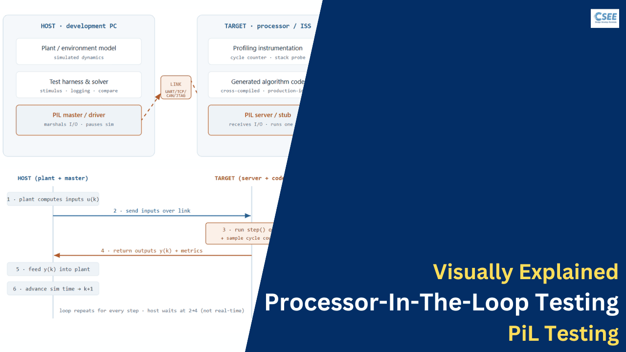
The host runs the plant model (the physics being controlled — a motor, a hydraulic actuator, a vehicle dynamics model), the test harness that injects stimulus and logs results, and the PIL master. The master is the piece that knows how to serialise the controller’s inputs, hand them to the link, wait for the target’s response, deserialise the outputs, and feed them back into the plant. It also pauses the solver while the target computes, which is precisely why PIL is not real-time.
Target side
On the target runs a small PIL server (sometimes called the target-side driver, stub, or harness) alongside the generated algorithm code. The server listens on the link, receives a set of inputs, calls the algorithm’s step function exactly once, optionally samples profiling instrumentation (a cycle counter, a stack watermark), and sends the outputs plus any metrics back. The algorithm code itself is the real production-intent object code, cross-compiled with the real toolchain.
The link
The communication channel can be a serial UART, a TCP/IP socket, a CAN bus, or a debugger connection over JTAG/SWD. It is deliberately abstracted: the algorithm never knows it is being driven by PIL, because the server sits between the link and the algorithm. This abstraction is what lets the same generated code run unchanged under PIL and in the shipped product.
The role of the plant model
The plant model deserves emphasis because its quality bounds what PIL can reveal. The controller’s inputs come entirely from this simulated plant, so if the plant never drives the controller into the operating regions where target-numeric defects hide — near saturation, at sign changes, at extreme setpoints — those defects will not appear no matter how faithful the target execution is. A rich, well-exercised plant model that visits the full operating envelope is therefore as important to PIL as the target setup itself. This is one reason back-to-back testing pairs PIL with deliberately edge-seeking test vectors: the plant plus the stimulus must jointly push the algorithm through its corner cases.
Why the split keeps results deterministic
A subtle but important property of this architecture is that the numeric results are independent of communication timing. Because the host pauses and waits for each target response before advancing simulated time, it does not matter whether a round trip takes one millisecond or one hundred — the sequence of inputs the algorithm sees, and the outputs it returns, are identical either way. This determinism is what lets PIL run on a slow serial link, a fast Ethernet link, or an in-process simulator and still produce exactly the same comparison against the baseline. The link affects only how long the test takes, never what it concludes.
Because the algorithm code is isolated behind the PIL server, PIL tests the exact object code you will ship, not a specially instrumented variant. Nothing about the algorithm is altered to make it testable — only the surrounding harness differs from production.
06 Inside one step
Anatomy of a single PIL simulation step
PIL runs as a lock-step co-simulation. For every solver step, control passes from host to target and back before simulated time advances. Tracing one step end-to-end is the clearest way to internalise how PIL works — and why it is slower than SIL but still numerically exact.
Step by step
- Plant produces inputs. The host solver evaluates the plant model for the current step and produces the input vector
u(k)the controller would see. - Marshal and transmit. The PIL master serialises
u(k)into the link’s byte format and sends it to the target’s PIL server. - Execute exactly one step on target. The server writes the inputs into the algorithm’s input structure, calls the generated
step()function once, and — if profiling is enabled — reads a cycle counter and stack watermark around that call. - Return outputs and metrics. The server serialises the algorithm outputs
y(k)plus any measured metrics and sends them back. - Feed the plant. The master deserialises
y(k)and applies it to the plant model as the controller’s actuation. - Advance time. The solver moves to step
k+1and the cycle repeats.
Initialisation and termination bracket the loop
The per-step loop is not the whole story. Before the first step, the target’s PIL server calls the algorithm’s initialise entry point once, setting states, integrators, and persistent buffers to their defined starting values — and any divergence in that initial state will propagate through every subsequent step, so it is verified too. After the final step, a terminate entry point may run to release resources. Bracketing the stepping loop this way mirrors exactly how the algorithm is invoked in the shipped product, where an initialise call precedes a periodic step task. PIL therefore verifies the same lifecycle the production scheduler will use.
Multi-rate models
Real controllers frequently run parts of the algorithm at different rates — a fast inner loop at 1 ms and a slower outer loop at 10 ms, say. Under PIL the co-simulation honours these rates: the appropriate rate’s step function is invoked when simulated time reaches its next sample instant, and the host solver coordinates which outputs are exchanged when. This means PIL faithfully reproduces multi-rate scheduling behaviour on the target, not just a single flat step — important because rate transitions and the sample-time hit logic are themselves places where generated code and target behaviour must agree.
Each round trip costs real milliseconds of communication, but simulated time only advances by one sample period regardless. Because the numeric results are unaffected by how long the transfer took, PIL stays bit-exact while running far slower than real time — a trade that is completely fine for correctness and static-timing verification.
07 The link
Communication channels and protocols
The physical link between host and target defines PIL’s setup complexity and throughput. There is no single “correct” choice — it depends on the board, the debug hardware you own, and whether you are running on real silicon or an instruction-set simulator. The table below compares the common options.
| Channel | Typical use | Speed | Setup effort | Notes |
|---|---|---|---|---|
| Serial / UART | Simplest boards, first bring-up | Low | Low | Universally available; slow but reliable |
| TCP/IP (Ethernet) | Boards with a network stack; ISS | High | Medium | Fast; needs an IP stack on target |
| CAN | Automotive ECUs already on a bus | Low–Medium | Medium | Reuses existing vehicle bus tooling |
| JTAG / SWD (debugger) | Via a probe (J-Link, TRACE32) | Medium | Medium | No target comms code; uses debug port |
| In-process (ISS) | Simulator, no hardware | High | Low | Fast function calls; no physical link |
Marshalling: turning signals into bytes
Whatever the channel, the master and server must agree on how each signal is packed into bytes — its data type, size, byte order, and position in the message. This is the marshalling or serialisation contract. Because the target’s endianness and alignment may differ from the host’s, the marshalling layer is itself a place where target-specific bugs can hide, which is another reason PIL is valuable: it exercises the real byte-level exchange, not an idealised one.
Target on real silicon vs an instruction-set simulator
You can run the “processor” half of PIL two ways. On real silicon (an evaluation board or the production MCU) you get true timing and true peripheral behaviour, at the cost of needing the hardware and a physical link. On an instruction-set simulator (ISS) — a cycle-approximate or cycle-accurate software model of the target core — you get the target’s numerics and an estimate of cycle counts without any board, which is ideal for early development and continuous integration. Many teams start PIL on an ISS and later repeat it on the physical board.
Throughput and test-suite duration
Because every step is a synchronous round trip, the link’s latency directly sets how long a PIL run takes. A test suite of a hundred thousand steps over a slow serial link can take many minutes; the same suite over Ethernet or on an ISS may finish in seconds. This is why channel choice is partly a productivity decision: a faster link does not change the results, but it changes whether PIL is pleasant to run on every commit or a chore reserved for milestones. Teams often keep a fast channel for routine regression and a slower, more representative board link for periodic confirmation.
Reliability over correctness
Whatever channel you pick, it must be lossless and ordered for the co-simulation to stay valid — a dropped or reordered message corrupts the input the algorithm sees and invalidates the comparison. Simple serial and TCP both provide this; a raw bus without a reliable transport layer needs framing and acknowledgement so no step is silently skipped. When PIL results look erratic across otherwise identical runs, an unreliable link is a prime suspect, ahead of the algorithm itself.
A common progression is: ISS-based PIL in CI for fast, hardware-free numeric checks → board-based PIL for true execution-time measurement → HIL for real-time integration. Each keeps the same generated code.
08 Granularity
What you can put in the loop — PIL scopes
PIL is not all-or-nothing. You choose how much of your design runs on the target versus on the host. Picking the right scope is a trade between fidelity, setup effort, and how much target memory the code fits into. Three common scopes appear across tools.
Top-model PIL
The entire controller model is generated, cross-compiled, and run on the target as one unit, driven by the top-level test harness. This gives the most complete on-target verification and the most representative timing, and is the natural choice once a subsystem is stable and fits the target’s memory.
Model-block / referenced-model PIL
A referenced model (a reusable component within a larger design) is placed in PIL mode while the rest of the model runs normally on the host. This lets you verify one component on the target while keeping the surrounding design fast and host-side — useful for large systems where only part of the code is ready for target testing.
Subsystem PIL
A specific subsystem is extracted, wrapped, generated, and run on the target. This is the finest-grained option: it isolates a single algorithm (say, a filter or a controller inner loop) for focused target verification and timing, with the least code to fit on the device.
| Scope | On target | Fidelity | Setup | Best for |
|---|---|---|---|---|
| Top-model | Whole controller | Highest | Higher | Final target sign-off + timing |
| Model block | One referenced model | High | Medium | Verifying a component in situ |
| Subsystem | One extracted subsystem | Focused | Lower | Isolating one algorithm early |
Start narrow (subsystem) to bring up the target connection and shake out numeric issues cheaply, then widen to top-model PIL once the whole controller is ready, so your final timing and coverage numbers reflect the complete algorithm.
09 Hands-on workflow
Setting up PIL in Simulink / Embedded Coder
The most widely used PIL implementation is the one in MathWorks Embedded Coder, so it is worth walking through concretely. The same conceptual steps — configure target, set up connectivity, switch the run mode, compare results — apply to other toolchains such as dSPACE TargetLink, only the buttons differ.
Step 1 — Configure the model for the target
Select an embedded system target file (for Embedded Coder this is ert.tlc) and set the hardware implementation to match the real device: device vendor and type, native word size, integer and pointer widths, byte ordering, and rounding behaviour. These settings tell the code generator to emit code whose arithmetic matches the target — and are what make the target’s numerics reproducible.
Step 2 — Set up target connectivity
The connectivity configuration tells Simulink how to build, download, and talk to the target: which cross-compiler and linker to invoke, how to deploy the binary, and which communication channel the PIL master and server will use. For supported boards this is provided by a hardware support package; for custom hardware you implement a connectivity configuration using the target-connectivity API, supplying a builder, a launcher, and a communicator.
Step 3 — Choose the PIL simulation mode
Set the run mode to Processor-in-the-Loop — either for the whole model (top-model PIL) or for a specific referenced model or subsystem block. This is the switch that redirects execution from the host to the target for the chosen scope.
Step 4 — Run
On run, the toolchain generates code for the selected scope, cross-compiles and links it with the PIL server, downloads the binary to the target (or launches the ISS), and executes the co-simulation step by step as described earlier. Signals stream back to the host for logging.
Step 5 — Compare against normal / SIL results
Finally, compare the PIL outputs against a trusted reference — the normal-mode (MIL) simulation or the SIL results — using a signal-comparison tool. Matching outputs (exactly for fixed-point, within tolerance for floating-point) demonstrate that the target code is equivalent. Divergence points you straight at a target-specific issue.
Step 6 — Read the report and iterate
A PIL run produces more than a pass/fail on outputs. It yields signal logs you can overlay against the baseline to see exactly where and when any divergence begins, plus the profiling report with per-step timing and resource figures. When outputs match, you record the run as equivalence evidence and move on. When they diverge, you use the first point of divergence to work backwards to the responsible operation — often a scaling, word-length, or rounding choice — adjust the model or its configuration, regenerate, and re-run. This tight loop of run, inspect, adjust, re-run is how target-specific issues get resolved while they are still cheap.
The same pattern in other tools
Although the walkthrough above uses Embedded Coder’s vocabulary, the shape is universal. In dSPACE TargetLink, for instance, the same block diagram can be exercised in MIL, SIL, and PIL modes, with the tool handling code generation, cross-compilation, download, and comparison. Whatever the environment, you are always answering the same three configuration questions — which device, how to reach it, and what scope to run there — and then comparing target results against a trusted reference. Learning the pattern once transfers across toolchains.
Configuring PIL is really three questions: what device (hardware implementation), how do I reach it (connectivity), and what scope runs there (top-model, model block, or subsystem). Answer those and the run is automatic.
10 Connectivity internals
Target connectivity — the three pieces you supply
For off-the-shelf boards, connectivity is handed to you by a support package. For custom silicon, you implement it yourself, and the abstraction breaks down into three responsibilities. Knowing them demystifies “why won’t PIL connect to my board.”
| Piece | Responsibility | Typically wraps |
|---|---|---|
| Builder | Cross-compile & link the generated code + PIL server for the target | Your cross-compiler, assembler, linker, makefile |
| Launcher | Download the binary and start it running on the target (or ISS) | Debugger/flash tool, board loader, simulator invocation |
| Communicator | Move bytes between host master and target server each step | Serial/TCP/CAN driver, or debugger memory access |
Builder
The builder invokes your production toolchain with the exact flags you will ship, compiling the generated algorithm together with the PIL server into a single downloadable image. Getting the builder right is what guarantees PIL exercises the real compiler and optimisation level — the whole reason PIL catches toolchain issues.
Launcher
The launcher gets that image onto the device: flashing it via a debug probe, loading it through a bootloader, or spawning the instruction-set simulator with the image as an argument. It also resets and starts execution so the server is ready to receive.
Communicator
The communicator implements the byte transport chosen in Table 7.1. On a debugger-based setup it may not use a serial line at all — it can read and write the target’s memory directly through JTAG, letting the host place inputs and read outputs without any target-side comms driver.
When PIL “hangs” or times out, the fault is almost always in the launcher or communicator, not the algorithm: wrong flash tool, wrong baud rate, a mismatched marshalling format, or the server never actually started. Verify the target boots and echoes on the link before blaming the generated code.
11 Proving equivalence
Back-to-back testing and numerical equivalence
The central deliverable of PIL is evidence of equivalence: proof that the target code produces the same results as the model and the host code. The technique is back-to-back testing — run identical stimulus through multiple stages and compare the outputs. When MIL, SIL, and PIL all agree on the same test vectors, you have a strong chain of evidence from algorithm to silicon.
Tolerance: exact vs approximate
How you compare depends on the arithmetic. For fixed-point designs, equivalence should be bit-exact — any difference is a real defect, because integer maths is deterministic. For floating-point designs, tiny differences can be legitimate: the target FPU, the order of operations chosen by the optimiser, or fused multiply-add can produce results that differ in the last bit. Here you compare within a small, justified tolerance and treat only larger divergences as failures.
| Design uses | Expected match | Any difference means |
|---|---|---|
| Fixed-point / integer | Bit-exact | A genuine defect — investigate |
| Floating-point | Within tolerance | Small: FPU/rounding order; Large: defect |
Where the test vectors come from
Good equivalence testing needs stimulus that exercises the design thoroughly, including edge cases: saturation limits, sign changes, zero crossings, and boundary values where overflow is most likely. Vectors can be authored by hand, captured from field data, or generated automatically by a formal test-generation tool that analyses the model and produces inputs achieving high structural coverage. Reusing the same vectors across MIL, SIL, and PIL is what makes the comparison meaningful.
Justifying a floating-point tolerance
When you compare floating-point outputs within a tolerance, that tolerance must be a reasoned value, not a number picked to make the test pass. A defensible tolerance is derived from the expected magnitude of legitimate differences — the unit in the last place of the data type, accumulated over the operation count of the algorithm, given the FPU and the compiler’s contraction behaviour. The discipline matters: too tight a tolerance produces false failures on harmless rounding differences; too loose a tolerance can mask a real defect. Document why the chosen tolerance is both large enough to admit legitimate FPU differences and small enough to catch genuine errors, and keep that justification alongside the test.
Kinds of test coverage the vectors should seek
Meaningful equivalence testing wants stimulus that reaches the design’s structural and behavioural corners. Useful categories include: boundary values at the edges of each signal’s range; saturation and overflow triggers that push accumulators to their limits; sign transitions and zero crossings where rounding and shift behaviour differs; mode and state transitions in any state machine; and structural-coverage vectors chosen so every branch, condition, and decision is exercised. A formal test-generation tool can analyse the model and synthesise inputs that drive uncovered branches, complementing hand-authored and field-captured vectors.
If MIL and SIL agree but PIL diverges, the code generator was faithful and the fault is target-specific — compiler, word size, or FPU. If SIL already diverged from MIL, the problem is in code generation, upstream of PIL. Comparing all three localises the defect to a single stage.
12 Reading the numbers
Execution profiling and on-target code metrics
Equivalence is one half of PIL’s value; the other is measurement. Because the code runs on the real processor, PIL can report resource figures no host-side test can produce. These numbers feed timing budgets, memory budgets, and safety arguments.
| Metric | What it tells you | Used for |
|---|---|---|
| Execution time / cycles | How long one step takes on the target | Schedulability, task time budgets |
| Max observed time | Longest step across all test vectors | Timing headroom (an empirical bound) |
| Stack usage | Peak stack depth reached | Preventing stack overflow |
| ROM (code) size | Flash the algorithm occupies | Fitting the device’s flash budget |
| RAM (data) size | Static + dynamic data footprint | Fitting the device’s RAM budget |
| Code coverage on target | Which branches executed on the device | Structural-coverage evidence (e.g. MC/DC) |
Execution time and the WCET caveat
PIL measures the observed execution time for the stimulus you ran. That is enormously useful — it tells you the algorithm’s real cost on the target and flags obvious budget problems early. It is not, however, a guaranteed worst-case execution time (WCET): a formal WCET bound requires static analysis that accounts for the paths and cache states your test vectors may never have triggered. Treat PIL timing as strong empirical evidence and a design signal, and pair it with dedicated WCET analysis where a hard guarantee is required.
Stack and memory
A stack-depth watermark sampled around the step call reveals the peak stack the algorithm used — vital on memory-constrained MCUs where a deep call chain or large local buffers can silently overflow into other data. Code and data size come from the map file the linker produces during the PIL build, giving you the true on-target footprint of production-intent code.
Structural coverage on the real binary
Collecting code coverage during PIL demonstrates which branches actually executed on the target, closing a subtle gap: coverage measured on host code does not, by itself, prove the target binary’s branches were exercised. For higher safety integrity levels, on-target structural coverage — including modified condition/decision coverage (MC/DC) — is part of the evidence set.
How the timing is actually measured
On most targets the execution-time figure comes from a free-running cycle counter — a hardware counter (such as a core debug cycle counter or a dedicated timer peripheral) that the PIL server samples immediately before and after the algorithm’s step call. The difference in counts, divided by the core clock, yields the step’s execution time. Because the sample brackets exactly the step function, the measurement excludes communication overhead and reflects only the algorithm’s cost. Where no cycle counter is available, a debugger-based setup can sometimes derive timing from trace, though at coarser resolution.
Interpreting the profile responsibly
Two habits keep timing data honest. First, report the maximum, not just the average — control tasks are budgeted against their worst step, and an average hides the occasional expensive path through a branch. Second, note the conditions: the optimisation level, the clock speed, and whether caches were enabled, since all three move the numbers substantially. A step time measured with optimisation off and caches disabled tells you little about shipped performance. Treat the PIL profile as a like-for-like measurement only when it is taken under production build settings.
Reading resource numbers against the budget
The value of ROM, RAM, and stack figures is entirely relative to the device budget. A 40 KB code size is comfortable on one MCU and impossible on another; a 900-byte peak stack is fine with a 4 KB stack and catastrophic with 1 KB. Good practice records each figure next to its device limit and the resulting headroom, so a reviewer sees at a glance not just the number but how close it sits to the ceiling. Trended over successive builds, shrinking headroom is the early-warning signal that a target is running out of room before it actually does.
A healthy PIL report shows outputs matching the baseline, max step time comfortably under budget, stack and memory within device limits, and coverage targets met on the target binary — all from a single automated run.
13 Ecosystem
Tools and toolchains used in PIL
PIL is a workflow, not a single product, so a real setup stitches together several tools: a model-based design environment that generates and orchestrates, a production cross-compiler, a debugger or probe to reach the target, an evaluation board or instruction-set simulator, and a comparison/reporting layer. The tables below map the ecosystem by role.
| Tool | Role in PIL |
|---|---|
| MATLAB / Simulink + Embedded Coder | Model design, production code generation, and built-in MIL/SIL/PIL run modes with connectivity API |
| Simulink Test | Authoring test cases and running back-to-back MIL/SIL/PIL comparisons |
| Simulink Design Verifier | Automatic test-vector generation for high structural coverage |
| dSPACE TargetLink | Fixed-point production code generation with its own MIL/SIL/PIL modes |
| ETAS / Vector toolchains | AUTOSAR-oriented code generation and integration workflows |
| Category | Examples | Why it matters for PIL |
|---|---|---|
| Cross-compilers | GCC (arm-none-eabi), IAR, Green Hills, TI, Wind River Diab, Keil | PIL exercises the real production compiler & flags |
| Debuggers / probes | Lauterbach TRACE32, SEGGER J-Link, vendor debug tools | Download, run, and often the comms channel via JTAG/SWD |
| Target boards / MCUs | Infineon AURIX, NXP, STM32, TI C2000, Renesas | The real silicon that provides true numerics & timing |
| Instruction-set simulators | Vendor ISS, third-party core models | Hardware-free PIL for early dev and CI |
| Static analysis | MISRA checkers, WCET analysers | Complement PIL with coding-rule & timing guarantees |
A typical automotive stack: Simulink/Embedded Coder or TargetLink generates and orchestrates, an IAR/Green Hills/GCC cross-compiler builds for the MCU, a TRACE32 or J-Link probe downloads and communicates, and the algorithm runs on an AURIX/NXP/STM32 board or its ISS — with results compared and reported back in the model environment.
14 Safety & standards
PIL in functional-safety and certification workflows
Much of PIL’s importance comes from safety standards that expect verification to continue all the way to the target. PIL provides the on-target equivalence and coverage evidence those standards ask for. It is rarely mandated by name, but it is the practical way teams satisfy the underlying requirement: show that the code that ships behaves as designed on the hardware it ships on.
| Standard | Domain | How PIL contributes |
|---|---|---|
| ISO 26262 | Automotive functional safety | Back-to-back model/code testing & on-target coverage evidence per ASIL |
| DO-178C | Airborne software | Object-code verification and structural coverage on the target |
| IEC 61508 | Industrial functional safety | Verification of the implemented software against its design |
| IEC 62304 | Medical device software | Evidence the target software matches the verified design |
| MISRA C / C++ | Coding guidelines | Applied to the generated code PIL then verifies on target |
Equivalence evidence for ASIL / DAL levels
Higher automotive integrity levels (ASIL C/D) and higher aerospace design assurance levels (DAL A/B) call for the strongest verification, including demonstrating that the object code executing on the target is a correct realisation of the requirements and design. Back-to-back MIL/SIL/PIL testing with matching outputs, together with on-target structural coverage such as MC/DC, is a well-established way to build that argument.
MISRA and generated code
MISRA C is a set of coding guidelines that restrict risky language constructs. Production code generators are configured to emit MISRA-compliant code, and PIL then verifies that this compliant code behaves correctly once compiled for the target — the two activities are complementary: MISRA governs how the code is written, PIL confirms that it runs correctly on the device.
Tool confidence and qualification
Because PIL relies on a code generator, a compiler, and a comparison tool, safety standards also care about how much you can trust those tools. Standards address this through concepts such as tool confidence levels and tool qualification: the more a tool’s output goes unchecked by other means, and the more severe an undetected tool error would be, the more evidence you need that the tool works as intended. PIL contributes here too — by independently checking that the generated, compiled code behaves as the model specified, it provides a detection mechanism that can lower the confidence burden on the generator, since a code-generation error would show up as a PIL divergence rather than slipping through unnoticed.
Building the evidence trail
What certification ultimately wants is a traceable argument from requirements to verified object code. PIL slots into that trail as the artefact demonstrating that the object code, on the target, satisfies the design that was itself traced to requirements. Kept as automated, repeatable runs with archived results — matching outputs, coverage figures, and resource measurements — PIL runs become durable evidence rather than one-off manual observations, which is exactly the form auditors and assessors expect to see.
No mainstream standard says the literal words “you must run PIL.” They require verification of the executable object code on the target and structural coverage of that code. PIL is the pragmatic, automatable technique most teams use to meet those requirements — which is why it is treated as near-mandatory at higher integrity levels even though it is not named.
15 Automation
PIL in continuous integration and regression testing
PIL delivers the most value when it runs automatically on every change, not just at milestones. Wired into continuous integration, PIL becomes a regression gate: any commit that alters the algorithm, the model configuration, the compiler flags, or the target settings triggers a fresh equivalence-and-timing check, and a divergence fails the build before it reaches a human.
Why ISS-based PIL shines in CI
Running PIL against an instruction-set simulator removes the hardware bottleneck: no board to share, no probe contention, and the run parallelises across build agents. You keep the target’s numerics and an estimate of timing while staying fully virtual. Teams then schedule periodic board-based PIL for true execution-time confirmation, keeping the fast virtual gate on every commit.
What to assert on
A robust PIL regression check does not only compare outputs. It should also fail the build when the maximum step time breaches its budget, when stack or memory exceeds the device limit, or when structural coverage drops below its target. Together these turn PIL from a one-off sign-off into a continuous guardrail against silent target-side regressions.
Automated PIL means a compiler upgrade, an optimisation-flag tweak, or a refactor that quietly changes target numerics is caught the same day it lands — not months later during HIL or, worst of all, in the field.
16 When it breaks
Common PIL problems and how to diagnose them
PIL setups fail in a handful of recognisable ways. Most are connectivity or configuration issues rather than algorithm bugs, and the symptom usually points at the cause. Use the table as a first-pass diagnostic.
| Symptom | Likely cause | First things to check |
|---|---|---|
| PIL hangs / times out on connect | Launcher or communicator misconfigured | Baud rate, flash tool, does the server start & echo? |
| Outputs diverge from baseline (fixed-point) | Target word-size overflow or scaling error | Accumulator widths, saturation, hardware-implementation settings |
| Outputs diverge slightly (floating-point) | FPU rounding / operation ordering | Is the difference within a justified tolerance? |
| Build fails during PIL | Cross-compiler flags or paths wrong | Toolchain in builder, include paths, target headers |
| Runs but no timing data | Profiling not enabled / no counter | Instrumentation option, target cycle-counter access |
| Stack overflow on target | Deep call chain or large locals | Stack watermark, reduce buffer sizes, increase stack |
| Code doesn’t fit the device | ROM/RAM budget exceeded | Map file, optimisation level, reduce scope to subsystem |
| Garbled values over the link | Marshalling / endianness mismatch | Byte order & type sizes agree host↔target |
Isolating a numeric divergence
Once you are confident the link and build are sound, a persistent output difference is a genuine numeric issue worth chasing carefully. The fastest route is to find the first step where PIL and the baseline diverge and inspect the internal signals feeding that step, because the earliest divergence is closest to the root cause; everything after it is downstream contamination. From there, suspect the usual culprits in order: accumulator and intermediate word lengths, saturation and rounding modes, and any operation whose result is implementation-defined. Reproducing the offending input in a tiny isolated model often makes the mechanism obvious. Resisting the urge to widen tolerances to make the symptom disappear is important here — a tolerance change hides the message without fixing the fault.
Work from the outside in: first prove the link works (the target boots and echoes), then prove the build is right (correct compiler and flags), and only then treat a persistent output difference as a genuine numeric defect. Most “PIL is broken” reports resolve at the first two layers.
17 Doing it well
Best practices for effective PIL testing
PIL rewards discipline. The teams that get the most from it treat it as a repeatable, automated stage with a clear reference baseline, not a manual checkbox performed once near tape-out. The practices below consistently separate smooth PIL adoption from painful ones.
Establish a trusted baseline first
PIL comparison is only as good as what you compare against. Lock down a verified MIL (and ideally SIL) baseline before you start, so a PIL divergence unambiguously indicates a target-specific issue rather than an unvalidated algorithm. Without a trusted reference, PIL differences are ambiguous and slow to diagnose.
Reuse identical stimulus across stages
Drive MIL, SIL, and PIL with the same test vectors. Shared stimulus is what makes back-to-back comparison meaningful and lets you localise a defect to the exact stage where divergence first appears. Different vectors per stage destroy that traceability.
Match the hardware-implementation settings to reality
The single most common source of spurious PIL divergence is a hardware-implementation configuration that does not match the true device — wrong word sizes, wrong endianness, wrong rounding. Set these precisely up front; they are the foundation of reproducible target numerics.
Prefer fixed-point exactness where you can
Fixed-point designs give you bit-exact comparison, which turns any difference into a crisp pass/fail signal. Where the design allows it, fixed-point makes PIL results unambiguous; where floating-point is required, pre-agree the tolerance and its justification.
Automate early and gate on it
Put PIL in CI from the start, ideally on an ISS for speed, and assert on outputs, timing, memory, and coverage together. Catching a target regression the day it lands is orders of magnitude cheaper than finding it at HIL. Manual PIL run once a quarter provides a fraction of the value.
Start small, then widen
Bring up the connection on a single subsystem to shake out launcher, communicator, and marshalling issues cheaply, then expand to top-model PIL for representative timing and complete coverage. Trying to stand up full top-model PIL on unproven connectivity is a common way to get stuck.
Record and trend the metrics
Keep the execution-time, stack, and memory numbers over time. A gradual creep in max step time or stack depth is an early warning that a control task is heading for its budget — visible only if you trend the data rather than glancing at a single run.
Trusted baseline · shared vectors · exact device settings · fixed-point where possible · automated in CI · start narrow then widen · trend the numbers. Do these and PIL becomes a quiet, reliable guardrail rather than a fragile milestone.
18 Honest limits
What PIL does not do
PIL is powerful but bounded. Knowing its limits is what tells you which verification job belongs to PIL and which belongs to another stage. Misplacing that boundary leads teams to expect guarantees PIL cannot give.
Not real-time, no real I/O
Because the host plant pauses while the target computes, PIL cannot verify real-time behaviour, interrupt timing under load, scheduler interactions, or the electrical behaviour of sensors, actuators, and drivers. Those are HIL’s job. PIL proves the algorithm is numerically correct and adequately fast per step, not that the fully integrated ECU meets its real-time deadlines with real signals.
Observed timing, not guaranteed WCET
PIL’s execution-time figures cover the paths your stimulus exercised. They are excellent early signals and empirical evidence, but they are not a formal worst-case bound. Where a hard timing guarantee is required, PIL must be complemented by static WCET analysis.
Slower than SIL
Communication overhead makes PIL markedly slower than SIL for the same test suite. This is rarely a correctness problem, but it does mean PIL is usually run on a curated, high-value vector set (or on an ISS) rather than on every conceivable input — you spend its slower cycles where target-specific risk is highest.
Setup complexity and hardware dependency
Board-based PIL needs the target, a probe, a working cross-toolchain, and correct connectivity — real infrastructure to stand up and maintain. ISS-based PIL removes the hardware but still requires an accurate core model. Neither is as frictionless as pressing “simulate” on the host.
It only sees what the stimulus drives
Like any dynamic test, PIL verifies only the behaviour your inputs actually provoke. A defect on a path no test vector reaches is a defect PIL will not report, however faithfully the target executes. This is why structural-coverage measurement is part of a serious PIL activity: coverage tells you which parts of the target binary your vectors truly exercised, and therefore how much of the code your equivalence evidence actually covers. High coverage plus matching outputs is strong evidence; matching outputs at low coverage is a much weaker claim, because most of the code was never run.
Mitigating the limits
None of these limits is a reason to skip PIL — each has a standard mitigation. Slow runs are addressed by ISS-based PIL and curated high-value vector sets. The lack of a guaranteed timing bound is addressed by pairing PIL’s empirical timing with static WCET analysis where a hard guarantee is needed. The absence of real-time and real I/O is addressed by the HIL stage that follows. Setup complexity is addressed by reusing hardware support packages and standing the connection up incrementally on a small scope first. Understood together, PIL’s limits simply define the seam between it and the neighbouring verification activities, each of which picks up precisely where PIL stops.
Use PIL for target numeric equivalence and static timing/resource measurement. Use HIL for real-time, real-I/O integration. Use static WCET tools for guaranteed timing bounds. PIL is one instrument in the verification kit, precise about a specific question — not a replacement for the others.
19 Reference
Glossary of PIL terms
| Term | Meaning |
|---|---|
| PIL / PiL | Processor-in-the-Loop: target code on the real processor, plant simulated on host |
| MIL | Model-in-the-Loop: controller and plant both simulated as models on the host |
| SIL | Software-in-the-Loop: generated code compiled for and run on the host |
| HIL | Hardware-in-the-Loop: real ECU driven in real time by a plant emulator with real I/O |
| Plant model | Simulated dynamics of the system being controlled (motor, vehicle, actuator) |
| PIL master | Host-side driver that marshals I/O and pauses the solver each step |
| PIL server / stub | Target-side harness that receives inputs, runs one step, returns outputs |
| Back-to-back testing | Running identical stimulus through multiple stages and comparing outputs |
| Cross-compiler | Compiler that builds on the host for a different target processor |
| ISS | Instruction-Set Simulator: software model of the target core, hardware-free |
| Marshalling | Serialising signals into the byte format exchanged over the link |
| WCET | Worst-Case Execution Time: a guaranteed upper bound (needs static analysis) |
| MC/DC | Modified Condition/Decision Coverage: a strong structural-coverage criterion |
| Fixed-point | Integer-based scaled arithmetic; deterministic, compared bit-exact |
| Hardware implementation | Config describing target word sizes, endianness, and rounding |
| ert.tlc | Embedded Coder’s embedded-real-time system target file |
| ASIL / DAL | Automotive / aerospace integrity levels driving verification rigour |
Putting it all together
Processor-in-the-Loop testing occupies a precise and valuable slot in the model-based verification chain. It is the moment the generated, production-intent code first meets the real target processor — proving, vector by vector, that the algorithm still computes what the model intended once the target’s word sizes, compiler, floating-point behaviour, and endianness are all in play, and measuring on the real device how long each step takes and how much memory and stack it consumes. It sits after SIL, which trusts the code generator on the host, and before HIL, which tests the fully integrated ECU in real time with real signals. Wired into continuous integration against a trusted baseline, with shared test vectors and device-accurate settings, PIL turns the risky gap between “compiles on my laptop” and “runs on the ECU” into a small, continuously guarded, well-instrumented step — which is exactly why it has become a near-mandatory practice wherever embedded software has to be both correct and safe.
Real code · real processor · simulated plant · compared to the model · measured on target. That five-part sentence is Processor-in-the-Loop testing in full.