Software-in-the-Loop Testing
A complete, visual, hands-on tutorial on how embedded control software is tested against a virtual world — the architecture, the closed loop, the workflow, the tools, and the engineering judgment behind it.
Imagine you have written the software that decides when a car should brake, how a drone should hold altitude, or when a battery pack should stop charging. Before that software ever touches a physical vehicle, aircraft, or battery, you want to know it behaves correctly — including in the dangerous situations you would never dare to stage in real life. Software-in-the-Loop (SiL) testing is how engineers do exactly that: they run the actual control software against a virtual model of the machine and its physics, and watch the two interact in a closed loop, thousands of times, for a fraction of the cost of a real test.
This tutorial builds your understanding from the ground up. We start with what SiL is and why it exists, place it inside the wider family of “X-in-the-Loop” techniques, then open up the architecture piece by piece. From there we walk through the closed loop, the signal flow, the workflow an engineering team actually follows, the tools they use, the standards they must satisfy, and the pitfalls that trip people up. Every major idea is paired with a diagram or a table, and everything is written to be read comfortably on a phone or a large monitor alike.
What this tutorial covers
- What SiL testing actually is
- Where SiL sits in the V-model
- The X-in-the-Loop family: MiL, SiL, PiL, HiL
- SiL architecture, layer by layer
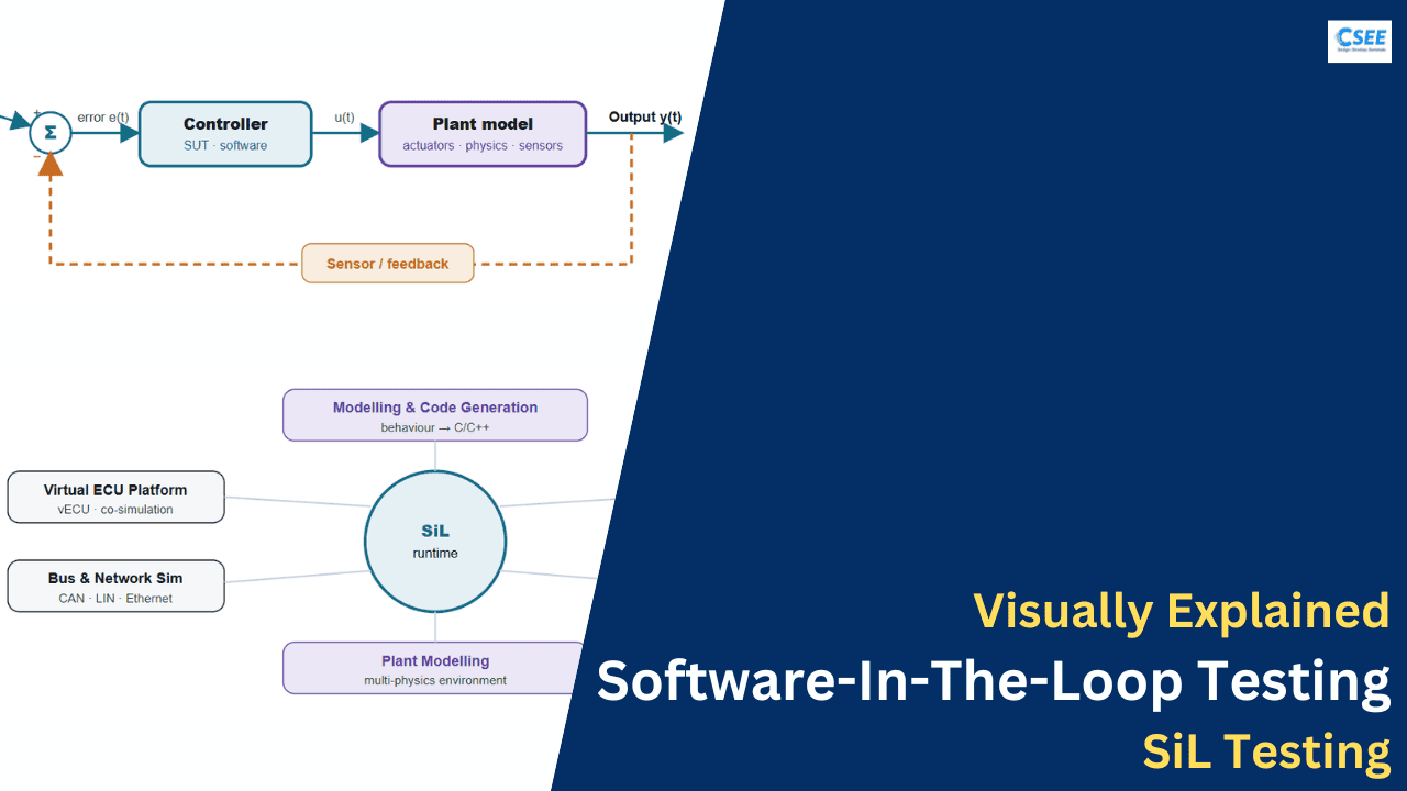
- The closed loop: controller and plant
- Signal flow and data exchange
- Open-loop vs closed-loop setups
- Core functions and components
- The SiL workflow, step by step
- Test design, coverage & back-to-back testing
- Tools and platforms
- Standards and compliance
- Advantages of SiL
- Limitations and challenges
- Best practices
- A worked example: cruise control ECU
- SiL in CI/CD and the cloud
- Metrics and KPIs
- Common pitfalls & fixes
- Glossary & FAQ
- SiL vs HiL in depth
- Plant-model fidelity levels
- Variants of SiL
- Getting started: a minimal setup
What SiL testing actually is
Definition · Core idea · Why it exists
Software-in-the-Loop testing is a verification technique in which the actual control software — the same logic that will eventually run inside a physical controller — is executed on a normal computer and connected to a simulated model of the system it is meant to control. Instead of wiring the software to real motors, valves, sensors, and a real vehicle, you wire it to a mathematical plant model that imitates how those things behave. The software and the model exchange signals continuously, forming a closed loop, and the whole thing runs as pure software on a host PC.
The name is worth unpacking. The “software” is the piece under test — the controller. The “loop” is the feedback loop between that controller and its environment. Putting the software “in the loop” simply means the real software is participating in a simulated control loop, driving a virtual machine and reacting to the virtual machine’s responses. Nothing about the machine is physical; everything is computed.
Why go to this trouble instead of just testing on real hardware? Because real hardware is slow to build, expensive to break, dangerous to push to its limits, and impossible to rewind. If you want to know how your battery-management software reacts when a cell suddenly overheats, you do not want to overheat a real battery a thousand times. In SiL you inject that fault in the model, watch the software respond, and repeat the scenario as often as you like — deterministically, at low cost, with every signal recorded.
The two halves of every SiL setup
Every SiL environment, no matter how elaborate, is built from two cooperating halves. The first is the System Under Test (SUT) — your control software. The second is the plant model — the simulated environment. A thin layer of “glue” connects them, converting one side’s outputs into the other side’s inputs and keeping their clocks in step.
What “real software” means here
A common point of confusion: is SiL testing the model of the software, or the final code? The honest answer is “either, and often both, at different moments.” Early in a project the controller exists only as a behavioural model — for example a Simulink or SCADE diagram. You can already put that model in the loop; some teams call this Model-in-the-Loop, but the closed-loop idea is identical. Later, that model is turned into C code by a code generator. Running that generated code in the loop is the classic, strictest sense of SiL, because you are now testing the artifact that will actually ship, compiled for the host but functionally identical to what runs on the target.
The key discipline is that the software’s behaviour must not change between the model, the generated code on the host, and the final code on the target. SiL is one of the checkpoints that proves this equivalence, which is why it forms such an important bridge in the development chain we will explore next.
Where SiL sits in the V-model
Development lifecycle · Verification checkpoints
To understand why SiL exists at a specific moment, it helps to see the development process it belongs to. Embedded and control systems are usually developed along a V-model: requirements and design flow down the left arm, implementation sits at the bottom, and testing climbs back up the right arm, with each test level verifying the design level directly across from it.
Reading the diagram, notice the natural order. On the left you refine what the system must do and how the software should be structured. At the bottom you implement — first as models, then as generated code. On the right you verify, and the technique you use depends on how close you are to real hardware. SiL lives near the bottom of the right arm, right after implementation, because that is the earliest moment the shippable software exists and the cheapest place to catch a defect.
This position matters economically. A defect found at the SiL stage costs a fraction of the same defect found during a physical system test, and orders of magnitude less than one found after production. Every rung you climb on the right arm makes each test slower, more expensive, and harder to reproduce. SiL’s job is to remove as many defects as possible while they are still cheap to remove — before the software is ever flashed onto a real controller.
The X-in-the-Loop family: MiL, SiL, PiL, HiL
The progression · What changes at each step
SiL is one member of a family of techniques known collectively as X-in-the-Loop (XiL). They all share the same closed-loop idea — a controller talking to a plant — but they differ in what plays the role of the controller and where that controller runs. Understanding the whole family clarifies exactly what SiL does and does not give you.
Reading the family from left to right
MiL (Model-in-the-Loop) tests the controller while it is still just a behavioural model. Everything — controller and plant — runs on the host inside the modelling tool. It is the earliest sanity check that your algorithm does the right thing in principle.
SiL (Software-in-the-Loop) replaces the controller model with the C/C++ code generated from it, compiled for the host. Now you are testing the actual implementation, catching bugs introduced by code generation, fixed-point arithmetic, integer overflow, and library differences — while still enjoying host-speed, fully virtual convenience.
PiL (Processor-in-the-Loop) takes that same code and cross-compiles it for the real target processor, then runs it on that processor (or an instruction-set simulator) while the plant stays on the host. This exposes compiler-and-CPU-specific effects: timing, word length, and target-specific numeric behaviour.
HiL (Hardware-in-the-Loop) goes all the way: the real electronic control unit, with real I/O electronics, is connected to a real-time simulator that plays the plant fast enough to fool the ECU into thinking it is in a real machine. This is the most realistic and most expensive rung below a physical prototype.
| Aspect | MiL | SiL | PiL | HiL |
|---|---|---|---|---|
| Controller is | Behavioural model | Generated C/C++ code | Target-compiled code | Real ECU firmware |
| Runs on | Host (modelling tool) | Host (compiled) | Target CPU / ISS | Real ECU hardware |
| Plant runs on | Host | Host | Host | Real-time simulator |
| Timing | Simulated | Simulated | Near-real / stepped | Hard real-time |
| Real I/O electronics | No | No | Partial | Yes |
| Cost | Very low | Low | Medium | High |
| Speed | Fast | Fast (often faster than real-time) | Moderate | Real-time only |
| Catches | Algorithm errors | Code-gen & numeric errors | Compiler/CPU effects | Electrical, timing, integration faults |
| Typical phase | Early design | Implementation | Pre-integration | System validation |
The crucial insight is that these techniques are complementary, not competing. A mature program runs all of them, escalating up the ladder. SiL is the workhorse in the middle-early zone: realistic enough to test production code, virtual enough to run overnight in the thousands. Because it needs no special hardware, SiL is also the rung that scales best in automated pipelines — a theme we return to in Section 17.
SiL architecture, layer by layer
The building blocks · How they stack
Let us now open the box and look at how a SiL environment is actually assembled. It helps to think in layers. At the top is the software you are testing. At the bottom is the model of the world. Between them sit the layers that make the two cooperate: interfaces, a co-simulation engine, a scheduler, and a harness that feeds in stimulus and records everything that happens.
What each layer does
Test harness & test manager
This top layer orchestrates the run. It selects which test cases to execute, drives the inputs (a braking manoeuvre, a temperature ramp, a fault injection), checks the outputs against expected results using assertions, and produces a report. It is the layer an engineer interacts with most directly.
System under test (SUT)
Your control software. In SiL this is typically the generated production code compiled into a shared library or executable, wrapped so the harness can call it every time step. It receives sensor-like inputs and produces actuator-like outputs, exactly as it would on the real controller.
Interface / adapter layer
Rarely do the controller’s signals line up perfectly with the plant’s. The adapter converts units and scaling, maps signal names, and abstracts communication buses (such as CAN, LIN, FlexRay, or Ethernet frames) into the plain variables each side understands. Getting this layer right is where a surprising amount of SiL effort goes.
Co-simulation engine & scheduler
Because the controller and the plant may be built in different tools with different solvers and different time steps, something must coordinate them. The co-simulation engine advances simulated time, decides the order in which tasks run, and exchanges signals at the agreed synchronisation points. In many setups this uses the open FMI (Functional Mock-up Interface) standard, packaging each side as an FMU (Functional Mock-up Unit).
Plant model
The virtual world: the physics of whatever the software controls, plus models of the sensors that report state and the actuators that carry out commands. Plant models range from simple lookup tables to high-fidelity multi-physics simulations.
Instrumentation
Cutting across every layer, instrumentation records signals, measures code coverage, and captures traces so that a failed test can be diagnosed and a passed test can be evidenced for certification.
The closed loop: controller and plant
Feedback control · Why the loop must close
The word “loop” is the heart of the whole idea, so it deserves its own section. In control engineering, a controller does not act blindly. It issues a command, observes the effect through sensors, compares the result against a desired target, and adjusts. This continuous cycle of act-observe-adjust is a feedback loop, and it is what SiL recreates in software.
Why the loop cannot be broken
You could, in principle, test a controller by feeding it a fixed recording of sensor values and checking its outputs. That is an open-loop test, and it has real uses (Section 7). But it cannot reveal how the controller behaves once its own actions change the world. A cruise controller that presses the throttle changes the vehicle’s speed, which changes the next sensor reading, which changes the next command. Only a closed loop — where the controller’s output genuinely influences the plant, which genuinely influences the next input — can expose instability, oscillation, overshoot, or a control law that quietly diverges.
This is why SiL insists on running the plant as a live, responsive model rather than a tape of pre-recorded signals. The plant must answer back. When the controller commands more torque, the virtual engine must actually produce more torque, the virtual vehicle must actually accelerate, and the virtual speed sensor must actually report the higher speed on the next step. The loop closes, and emergent behaviour becomes visible.
The controller side in detail
The controller in SiL is your production logic. It might implement a PID law, a state machine, a lookup-table-based calibration, a model-predictive optimiser, or a supervisory mode manager. Whatever its internals, from the loop’s point of view it is a function: given the current inputs (setpoints, sensor readings, bus messages, diagnostics), produce outputs (actuator commands, status flags, bus messages) — every time step.
The plant side in detail
The plant must model three things: the actuators that turn commands into physical effects, the process or physics that evolves over time, and the sensors that measure the process and report it back — ideally including sensor imperfections such as noise, delay, quantisation, and range limits. A plant that is too perfect will let buggy software pass; a plant with realistic imperfections stresses the controller the way reality will.
Signal flow and data exchange
Time stepping · Co-simulation · FMI/FMU
We have seen the layers and the loop. Now let us follow a single simulation step in detail, because the timing of the data exchange is where SiL setups succeed or subtly fail. In each step the two halves must exchange the right values in the right order, and simulated time must advance consistently for both.
Fixed step, variable step, and rate handling
The controller almost always runs at a fixed step — for instance every 10 milliseconds — because that is how it will run on the real target, driven by a periodic task. The plant, by contrast, may prefer a variable-step solver that takes small steps through fast transients and large steps through calm stretches, for accuracy and speed. The co-simulation engine reconciles these, ensuring the controller sees a consistent 10 ms cadence while the plant integrates as finely as it needs between exchanges. Multi-rate systems — where different controller tasks run at different periods — add another layer the scheduler must respect.
Co-simulation and the FMI standard
When the controller and plant come from different tools, they are frequently exchanged as Functional Mock-up Units (FMUs) conforming to the Functional Mock-up Interface (FMI) standard. An FMU is a self-contained package — compiled model code plus an interface description — that any FMI-compatible tool can load and step. This decouples the SiL environment from any single vendor: a plant modelled in one tool and a controller generated by another can meet on neutral ground.
Open-loop vs closed-loop setups
Two testing modes · When to use each
Although the closed loop is the defining feature of SiL, engineers deliberately use two modes, and knowing when to choose each is part of the craft.
Open-loop testing
In open-loop mode, the controller’s outputs do not feed back to change its inputs. Instead you drive the controller with predetermined input sequences — often recorded from a real drive, a test rig, or a requirement specification — and check that its outputs match expectations. It is simple, perfectly repeatable, and excellent for verifying discrete logic, calculations, diagnostics, and requirement-by-requirement checks. What it cannot show is dynamic stability, because the world never reacts.
Closed-loop testing
In closed-loop mode, the plant model is live and the controller’s actions genuinely change future inputs. This is the mode that reveals overshoot, limit cycles, controller wind-up, mode-switching glitches, and interactions between multiple control functions. It is more expensive to set up because you must build and validate a plant model, but it is the only way to test the controller as a participant in real dynamics.
| Dimension | Open-loop | Closed-loop |
|---|---|---|
| Plant model | None (recorded/stubbed inputs) | Live, responsive plant |
| Controller output affects input? | No | Yes |
| Best for | Logic, math, diagnostics, requirement checks | Dynamics, stability, control quality |
| Repeatability | Exact | Exact (deterministic) |
| Setup effort | Low | Higher (needs plant) |
| Reveals instability? | No | Yes |
| Typical use | Unit & requirement tests | Function & integration tests |
Most projects use both: open-loop for fine-grained, requirement-traceable checks of individual behaviours, and closed-loop for the emergent, dynamic behaviour that only appears when the controller and its world influence each other. The two modes together give both precision and realism.
Core functions and components
The parts inventory · Responsibilities
Beyond the high-level layers, a working SiL environment is made of concrete components, each with a job. Here is the practical inventory you will encounter when you build or inherit one.
How the components collaborate
During a run, the stimulus generator and any fault injector shape the scenario. Each step, the scheduler asks the SUT to compute; the interface adapter passes commands through actuator models into the plant; the plant evolves and its state is read back through sensor models and bus models; the assertion checks the outcome; and the logger records everything. When the scenario ends, the report generator assembles the evidence. Every one of these can be swapped independently, which is what makes SiL environments so reconfigurable.
The SiL workflow, step by step
From requirement to report · The pipeline
Building and running SiL is a repeatable process. The pipeline below is the arc most teams follow, whether by hand early on or fully automated later.
Stage by stage
1. Requirements. Every test must trace to a requirement. Before anything else, capture what “correct” means: response times, tolerances, safety reactions, mode behaviour.
2. Plant model. Build (or reuse) a model of the environment at the fidelity the requirements demand, and validate it against measurements or first principles so you trust its answers.
3. Generate code. Turn the controller model into C/C++ with a qualified code generator and compile it for the host. This is the step that turns MiL into true SiL.
4. Integrate. Connect the SUT and plant through the interface adapter, resolve signal mappings and rates, and confirm the loop runs stably before you trust its results.
5. Test cases. Design scenarios and their oracles — the expected outcomes. Cover nominal operation, boundaries, and fault conditions.
6. Execute. Run the closed loop across all scenarios, ideally in batch, capturing every signal.
7. Assess. Compare outcomes to oracles, measure code and requirement coverage, and flag failures.
8. Report. Produce traceable evidence linking each requirement to the tests that verify it — indispensable for safety certification.
The dashed return path is the point: SiL is iterative. Failures feed fixes, fixes trigger re-runs, and because the whole loop is virtual, that cycle can spin many times a day.
Test design, coverage & back-to-back testing
What to test · How much · Proving equivalence
Running the loop is only half the work; deciding what to run and how thoroughly is the other half. Three ideas dominate: scenario design, coverage, and back-to-back testing.
Designing test scenarios
Good SiL scenarios come from four sources. Requirements give the must-pass behaviours. Boundary analysis pushes inputs to their limits and just beyond — the edges where bugs hide. Equivalence partitioning groups inputs that should behave alike so you test one representative from each group instead of every value. And fault scenarios deliberately break sensors, actuators, and messages to confirm the software’s safety reactions. A balanced suite mixes all four, plus long “mission” runs that expose slow drift and accumulation errors.
Measuring coverage
Coverage answers “how much of the software did the tests actually exercise?” Structural coverage metrics increase in strictness, and safety standards demand stronger metrics for more critical software.
| Metric | What it requires | Strength |
|---|---|---|
| Statement | Every line of code executed at least once | Basic |
| Branch / Decision | Every decision takes both true and false outcomes | Moderate |
| Condition | Every boolean sub-condition takes both values | Strong |
| MC/DC | Each condition independently shown to affect the decision | Very strong |
| Function / Call | Every function and every call site invoked | Basic |
MC/DC (Modified Condition/Decision Coverage) is the demanding metric required for the most critical software in aerospace (DO-178C level A) and high-integrity automotive functions. It is far harder to achieve than statement coverage, which is exactly why teams pursue it in SiL, where creating the necessary corner-case inputs is cheap and repeatable.
Back-to-back testing: proving equivalence
One of SiL’s most valuable roles is back-to-back testing — running the same scenarios through the model (MiL) and through the generated code (SiL) and confirming the outputs match within tolerance. If they match, you have evidence the code generator preserved the model’s behaviour. If they diverge, you have found a code-generation, data-typing, or numeric bug before it ever reached hardware.
Tools and platforms
The ecosystem · What each tool does
SiL is supported by a rich tool ecosystem. Broadly the tools fall into five roles: modelling & code generation, test authoring & execution, virtual ECU / co-simulation platforms, plant modelling, and coverage & static analysis. The map below shows how they fit together; the table lists representative products.
| Role | Representative tools | What it contributes to SiL |
|---|---|---|
| Modelling & code-gen | MATLAB/Simulink + Embedded Coder, ANSYS SCADE, dSPACE TargetLink | Author control logic and generate production C/C++ for the SUT |
| Test authoring | Simulink Test, dSPACE AutomationDesk, Vector vTESTstudio, BTC EmbeddedPlatform | Create scenarios, oracles, and requirement-linked test suites |
| Virtual ECU / co-sim | dSPACE VEOS, Synopsys Silver, ETAS COSYM/ISOLAR-EVE, Vector vVIRTUALtarget | Host the vECU and orchestrate co-simulation of controller and plant |
| Plant modelling | Simscape, GT-SUITE, AVL, Modelica tools, IPG CarMaker | Provide physics-based environment and vehicle dynamics |
| Bus / network | Vector CANoe, dSPACE bus models | Emulate CAN/LIN/FlexRay/Ethernet communication |
| Coverage | BTC EmbeddedTester, LDRA, VectorCAST, Simulink Coverage | Measure statement/branch/MC/DC coverage of the SUT |
| Static analysis | Polyspace, MISRA checkers, Coverity | Find defects and coding-rule violations before execution |
| Interchange | FMI/FMU tooling | Package and exchange models across tools vendor-neutrally |
Standards and compliance
Why SiL is often mandatory · Key standards
In safety-critical domains, testing is not optional and neither is the evidence that it was done. Several standards effectively require the kind of early, traceable, coverage-measured verification that SiL provides. Understanding them explains much of why SiL is structured the way it is.
| Standard | Domain | Relevance to SiL |
|---|---|---|
| ISO 26262 | Automotive functional safety | Requires verification at unit and integration level with coverage evidence; SiL supplies it early and repeatably (ASIL A–D). |
| ISO 21448 (SOTIF) | Automotive intended function | Encourages scenario-based testing of performance limitations; SiL enables mass scenario exploration. |
| Automotive SPICE | Automotive process quality | Demands traceability from requirements to tests; SiL reports provide the linkage. |
| DO-178C | Airborne software | Mandates structural coverage up to MC/DC for the highest levels; SiL is a primary means to achieve it. |
| IEC 61508 | Industrial functional safety | General functional-safety umbrella; SiL supports required verification activities. |
| MISRA C/C++ | Coding guidelines | Restricts risky language constructs; checked on the SUT code that SiL executes. |
| FMI | Model interchange | Enables vendor-neutral co-simulation, easing tool qualification and reuse. |
The recurring themes
Read across the table and three demands repeat. First, traceability: every requirement must be verifiable, and every test must link back to a requirement. Second, coverage: the more critical the software, the stronger the structural coverage you must demonstrate, up to MC/DC. Third, tool confidence: the tools that generate code and measure results must themselves be qualified or their output independently confirmed. SiL directly serves all three — it exercises production code against requirement-linked scenarios while measuring coverage, and back-to-back testing helps confirm the code generator behaved.
Advantages of SiL
Why teams invest in it
SiL’s advantages all flow from one fact: the entire loop is software. That unlocks a cluster of benefits no hardware-based method can match at the same cost.
Early defect detection
Because SiL runs the moment generated code exists, defects are caught while they are cheapest to fix — long before any prototype. This is the economic core of the technique.
Safety without danger
You can test the exact scenarios that would be reckless or impossible in reality — brake failure at speed, sensor loss on final approach, thermal runaway — because nothing physical is at risk.
Speed and scale
Freed from real-time constraints, SiL can often run faster than real-time and in parallel across many machines, executing thousands of scenarios overnight.
Perfect repeatability
A virtual loop is deterministic. A failing scenario reproduces exactly, every time, which makes debugging dramatically easier than chasing an intermittent hardware fault.
Full observability
Every internal signal is visible and loggable, with no probes, no wiring, and no measurement noise. You can see states that are physically inaccessible on real hardware.
Cost efficiency
No test benches, no prototypes, no consumables. The marginal cost of one more test is essentially compute time.
Automation friendliness
Because it needs no special hardware, SiL slots directly into continuous-integration pipelines, running automatically on every code change (Section 17).
Shift-left leverage
SiL lets teams verify production code before hardware exists, compressing schedules and de-risking the expensive later stages.
Limitations and challenges
Where SiL stops · Honest caveats
SiL is powerful but not complete. Its limitations are the mirror image of its strengths, and respecting them is what keeps a verification strategy honest.
Only as good as the plant model
SiL tests the controller against a model of reality. If the plant model is wrong or too simplified, the software can pass in simulation and fail in the world. Plant validation is therefore a first-class activity, not an afterthought.
No real timing or hardware effects
Running on the host, SiL does not reveal real-target execution time, interrupt latency, memory constraints, or compiler-specific behaviour. Those need PiL and HiL.
No electrical or physical faults
Short circuits, connector corrosion, electromagnetic interference, voltage sag, and sensor wiring faults live in the physical world. SiL can model their logical effects but not the electrical reality.
Modelling effort and cost
A high-fidelity plant model can take as long to build and validate as the controller itself. That investment is the price of admission for closed-loop testing.
Risk of over-trust
A polished green SiL report can create false confidence. SiL reduces risk; it does not eliminate the need for HiL and real-world validation.
Co-simulation pitfalls
Mismatched step sizes, signal-exchange delays, and solver interactions can produce artefacts that look like software bugs but are really integration errors — subtle and time-consuming to diagnose.
Best practices
Hard-won guidance
Teams that get lasting value from SiL tend to share a set of habits. None are exotic; together they separate a durable test asset from a brittle one.
- Never modify the SUT for the test. All adaptation lives in the interface layer. The instant you tweak the control code to fit the rig, you are no longer testing what ships.
- Validate the plant before trusting the loop. Compare the plant model against measurements or analytic expectations. An unvalidated plant produces confident nonsense.
- Match fidelity to the requirement. Model finely only where correctness depends on it. Uniform high fidelity wastes effort and slows runs.
- Trace every test to a requirement. Untraceable tests cannot serve certification and tend to rot. Bidirectional traceability keeps the suite meaningful.
- Reuse one harness across MiL and SiL. A shared harness makes back-to-back testing trivial and keeps model and code honest with each other.
- Automate execution. Wire SiL into CI so it runs on every change. Manual SiL decays; automated SiL compounds.
- Version everything together. Plant model, SUT, scenarios, and tolerances must be versioned as a set, or results become impossible to reproduce.
- Keep tolerances explicit and reviewed. Back-to-back and reference comparisons need documented, justified tolerances, not magic numbers buried in a script.
- Inject faults deliberately. Nominal-only suites miss the safety reactions that matter most. Build a fault catalogue and exercise it.
- Treat coverage as a guide, not a goal. High coverage with weak oracles proves little. Coverage tells you where you have not looked; strong assertions tell you whether what you looked at was right.
A worked example: cruise control ECU
Concrete walk-through · Signals, scenarios, verdicts
Abstract ideas settle once you watch them applied. Let us put a simple adaptive-style cruise control function through SiL, end to end. The controller’s job: hold a driver-set speed, and ease off if a slower lead vehicle appears.
The signals
| Direction | Signal | Meaning |
|---|---|---|
| in | v_set | Driver’s target speed |
| in | v_ego | Measured own-vehicle speed (from plant) |
| in | d_lead | Distance to lead vehicle (from plant) |
| in | enable | Cruise on/off switch |
| out | a_req | Requested acceleration to actuators |
| out | status | Active / standby / fault flag |
The plant model
The plant integrates a straightforward longitudinal vehicle model: requested acceleration, minus drag and grade, gives actual acceleration, which integrates to speed and position. A lead-vehicle sub-model drives d_lead. Sensor models add noise and a small delay to v_ego and d_lead so the controller faces realistic imperfection.
The scenarios and verdicts
| # | Scenario | Expected controller behaviour | Verdict logic |
|---|---|---|---|
| T1 | Set 100 km/h on empty road | Accelerate smoothly, settle at 100, no overshoot > 3% | Overshoot & steady-state error within tolerance |
| T2 | Slower lead vehicle appears | Reduce speed, keep safe gap | Min gap never below threshold |
| T3 | Lead vehicle clears | Resume set speed | Returns to v_set within time budget |
| T4 | Steep uphill grade | Hold speed, no divergence | Speed stays within band on grade |
| T5 | v_ego sensor freezes (fault) | Detect fault, enter safe standby | status = fault within reaction time |
| T6 | Driver disables mid-manoeuvre | Release control cleanly | a_req → 0, no jerk spike |
Notice the mix: T1–T4 test nominal dynamics in closed loop, T5 injects a fault to confirm the safety reaction, and T6 checks a mode transition. Each has a crisp, automatable verdict tied to a requirement — no human judgment needed at run time.
What SiL reveals here
Run T1 and you might discover the controller overshoots because a gain is too aggressive — visible instantly as the speed trace sails past 100 and rings back. Run T5 and you might find the fault takes one step too long to latch, breaching the reaction-time requirement. Both are the kind of dynamic, timing-sensitive defect that open-loop checks would miss and that would be expensive to reproduce on a real vehicle — caught here, on a laptop, in seconds, and reproducible on demand.
SiL in CI/CD and the cloud
Automation · Scale · Modern trends
SiL’s biggest modern advantage is that, needing no hardware, it fits naturally into continuous integration and continuous delivery (CI/CD). Every time an engineer changes the control software, a pipeline can regenerate code, rebuild the SiL environment, run the full scenario suite, measure coverage, and publish a report — automatically, within minutes, on a build server or in the cloud.
Why this matters
Automated SiL turns verification from an event into a continuous background process. Regressions are caught the moment they are introduced, while the change is fresh in the author’s mind. Because runs are parallelisable and hardware-free, a cloud fleet can execute enormous scenario libraries — the “millions of virtual miles” approach central to modern driver-assistance and autonomy programs.
The virtual ECU and the software-defined vehicle
A strong trend is the virtual ECU (vECU): a complete software image of a controller — application, middleware, and sometimes operating system and basic software — running on the host. vECUs push SiL closer to the real firmware without needing the chip, and they underpin the software-defined vehicle, where large fleets of virtual ECUs are integrated and tested entirely in the cloud before any silicon is involved.
Metrics and KPIs
Measuring a SiL program’s health
A SiL effort should be measured, not just performed. The indicators below tell you whether the program is genuinely reducing risk or merely producing green lights.
| KPI | What it tells you | Healthy direction |
|---|---|---|
| Requirement coverage | Share of requirements with at least one passing test | → 100% |
| Structural coverage | Code exercised (statement/branch/MC/DC) | → target for the safety level |
| Back-to-back pass rate | Model vs code agreement within tolerance | High & stable |
| Defect escape rate | Bugs found later (HiL/field) that SiL could have caught | → 0 |
| Suite run time | Wall-clock to run the full suite | Low (enables frequent runs) |
| Flakiness | Tests with non-deterministic results | → 0 (SiL should be deterministic) |
| Fault-scenario share | Proportion of tests exercising fault reactions | Meaningful, not token |
| Plant validation status | Confidence the plant matches reality | Documented & current |
Two KPIs deserve emphasis. Defect escape rate is the ultimate scorecard: if defects that SiL could have caught keep surfacing at HiL or in the field, the suite’s oracles or scenarios are too weak, regardless of how green the dashboard looks. And flakiness should be essentially zero — a virtual, deterministic loop that produces different results on re-runs signals a co-simulation or ordering bug that must be fixed before any result can be trusted.
Common pitfalls & fixes
Troubleshooting field guide
Most SiL frustration comes from a handful of recurring traps. Recognising the symptom shortens the hunt considerably.
| Pitfall | Typical symptom | Remedy |
|---|---|---|
| Feedback delay in exchange | Stable design oscillates only in SiL | Check signal-exchange ordering; align controller and plant step timing |
| Over-simplified plant | Passes SiL, fails HiL or field | Raise fidelity where correctness depends on it; validate against data |
| Weak oracles | High coverage, defects still escape | Strengthen assertions; tie verdicts to real requirement thresholds |
| Tolerance too loose | Back-to-back never fails, even on real bugs | Tighten and justify tolerances; review them |
| Tolerance too tight | Back-to-back fails on normal numeric noise | Set tolerance to expected fixed/float difference |
| Modified SUT | Test passes but real code differs | Move all adaptation into the interface layer |
| Unversioned assets | Results cannot be reproduced later | Version SUT, plant, scenarios, tolerances together |
| Non-deterministic run | Same test, different results | Remove wall-clock/random dependence; fix task ordering |
| Rate mismatch | Aliasing or missed events | Respect multi-rate scheduling; sample fast enough |
| No fault scenarios | Safety reactions untested | Build and run a fault-injection catalogue |
Glossary & FAQ
Quick reference · Common questions
Glossary
Frequently asked questions
Is SiL the same as unit testing?
No, though they overlap. Unit testing usually checks small pieces in isolation with fixed inputs. SiL exercises the integrated control software in a closed loop against a dynamic plant, revealing behaviour that unit tests cannot — though SiL can host unit-level checks too.
Does SiL replace HiL?
No. They answer different questions. SiL verifies software logic and control behaviour cheaply and early; HiL verifies real timing, electrical I/O, and hardware integration. A complete program uses both, escalating from SiL to HiL.
Can SiL run faster than real time?
Often yes. Because it is unconstrained by physical clocks, a SiL loop can simulate minutes of behaviour in seconds, which is what makes large-scale, overnight scenario sweeps practical.
What makes a SiL result trustworthy?
Three things: a validated plant model, strong requirement-linked oracles, and reproducibility. Without a trustworthy plant and meaningful assertions, a green result proves little.
Do I need generated code, or can I use hand-written code?
Either. SiL applies to any control software you can compile for the host, whether model-generated or hand-written. The technique is about the closed loop, not the code’s origin.
Where does SiL fit for autonomous systems?
Centrally. Driver-assistance and autonomy rely on massive, cloud-scale scenario testing that only virtual, hardware-free methods like SiL can deliver at the required volume — millions of virtual situations, replayed deterministically.
How much of my test effort should be SiL versus HiL?
There is no universal ratio, but the guiding principle is clear: push every check that does not genuinely require hardware down into SiL, and reserve HiL for real timing, electrical integration, and final system validation. In practice this often means the large majority of functional test cases run in SiL, executed continuously, while a smaller, carefully chosen set graduates to HiL. If you find HiL surfacing basic logic defects, your SiL suite is too thin and should be strengthened rather than your HiL time expanded.
What skills does a SiL engineer need?
A blend. You need enough control-systems literacy to reason about loops, stability, and dynamics; enough software skill to build harnesses, adapters, and automation; enough modelling knowledge to judge plant fidelity; and enough testing discipline to write meaningful oracles and trace them to requirements. The rarest and most valuable habit, though, is skepticism — the reflex to distrust a suspiciously green result and to keep asking what the test has not yet proven.
SiL vs HiL in depth
The most important comparison · When to escalate
Of all the XiL techniques, the pair engineers most often weigh against each other is SiL and HiL. They sit at opposite ends of the cost-realism trade-off, and choosing how much to invest in each shapes an entire verification strategy. It is worth slowing down to understand exactly how they differ and, more importantly, how they complement each other.
The fundamental distinction is what is real. In SiL, nothing physical exists: the controller is compiled code on a host, and the plant is a mathematical model on the same host. In HiL, the controller is the genuine electronic control unit — the real circuit board, the real microcontroller, the real firmware, the real input and output electronics — connected to a real-time simulator powerful enough to imitate the plant fast enough that the ECU cannot tell it is being fooled. HiL therefore tests things SiL structurally cannot: the behaviour of real analog-to-digital converters, the timing of interrupts on the actual silicon, the electrical characteristics of sensor and actuator drivers, the effect of supply-voltage variation, and the integration of the ECU with real communication transceivers.
But that realism has a price, and the price is exactly what makes SiL attractive. HiL requires the physical ECU to exist, which means it cannot begin until hardware is available — often late in a project. It requires an expensive real-time simulator and custom wiring for every signal. It runs only at real-time speed, so a scenario that takes ten minutes in the world takes ten minutes on the bench; you cannot fast-forward. It is harder to reproduce exactly, because real electronics introduce small variations. And it does not scale cheaply: running a thousand scenarios means a thousand real-time executions on a scarce, costly bench, whereas SiL can spread the same thousand scenarios across a fleet of ordinary computers and finish before lunch.
How they divide the work
The mature answer is not to choose but to sequence. SiL carries the enormous bulk of functional verification — the logic, the control laws, the mode management, the fault reactions, the requirement-by-requirement checks, the regression suite that runs on every commit. By the time a function reaches HiL, its software behaviour should already be trusted, so HiL can concentrate on what only it can test: real timing, real electrical integration, and the emergent behaviour of the complete physical controller. Framed this way, SiL is not a weaker HiL; it is the filter that lets the expensive HiL bench spend its scarce hours on the questions that genuinely require hardware.
| Question | SiL | HiL |
|---|---|---|
| When can it start? | As soon as code is generated | Only once the ECU hardware exists |
| What is real? | Nothing (all software) | The ECU + its I/O electronics |
| Execution speed | Often faster than real-time | Real-time only |
| Scales to thousands of runs? | Yes, cheaply, in parallel | No, bench-bound |
| Reveals real timing/interrupts? | No | Yes |
| Reveals electrical faults? | No (only logical effects) | Yes |
| Reproducibility | Exact / deterministic | Very high, with minor variation |
| Cost per additional test | Compute time only | Bench time + operator |
| Fits CI on every commit? | Yes | Rarely (nightly at best) |
| Primary purpose | Verify software behaviour early | Verify hardware/software integration |
Plant-model fidelity levels
How real should the virtual world be?
The single decision that most determines whether a SiL environment is useful or misleading is how much fidelity to build into the plant model. Fidelity is not free — every increment costs modelling effort, validation effort, and simulation time — so choosing the right level for each question is a core engineering skill rather than a matter of “more is better.”
It helps to think of fidelity as a ladder. At the lowest rung sits the functional or behavioural model: it captures the input-output relationship of the plant just well enough to close the loop, often with lookup tables and first-order lags. It is fast, easy to build, and perfect for early logic testing where you only need the world to respond in roughly the right direction. Its danger is that it can flatter the controller, hiding problems that a more realistic world would expose.
The middle rung is the physics-based model, where real conservation laws govern the behaviour: forces, masses, energies, flows, and thermodynamics are modelled from first principles. A physics-based vehicle model computes acceleration from actual force balance rather than a curve fit, so it behaves correctly even in situations the modeller never explicitly anticipated. This is the level at which closed-loop dynamic testing becomes genuinely trustworthy, and it is where most serious control verification lives.
The top rung is the high-fidelity, multi-physics model, which couples several domains — mechanical, electrical, thermal, hydraulic, chemical — and adds fine detail such as component nonlinearity, saturation, hysteresis, temperature dependence, and detailed sensor and actuator imperfections. These models can rival the controller in complexity and cost, so they are reserved for the questions that truly demand them: the last few percent of control quality, edge-of-envelope behaviour, or safety cases where an optimistic plant would be unacceptable.
| Level | What it captures | Best for | Cost |
|---|---|---|---|
| Behavioural | Rough input-output response, tables, lags | Early logic & mode testing | Low |
| Physics-based | First-principles dynamics | Trustworthy closed-loop control tests | Medium |
| Multi-physics | Coupled domains, nonlinearity, detail | Edge cases, safety cases, final tuning | High |
| Sensor/actuator detail | Noise, delay, drift, saturation, faults | Robustness & diagnostics testing | Medium |
Mixing fidelity within one model
Real environments rarely use a single level everywhere. A skilled modeller raises fidelity only along the paths the controller’s correctness actually depends on, and keeps everything else cheap. If the software under test cares intensely about wheel-slip but barely about cabin temperature, the tyre model earns high fidelity while the thermal model stays behavioural. This selective investment is what keeps a high-value plant model affordable and fast enough to run in the thousands.
Variants of SiL
Not one technique but a family of setups
“SiL” is an umbrella. Under it live several concrete setups that differ in what plays the controller, how many controllers participate, and how much of the software stack is included. Recognising the variant you are using clarifies what your results actually prove.
Model-against-model
Both controller and plant are behavioural models running in the same environment. Strictly this is the MiL end of the spectrum, but it shares SiL’s harness and scenarios and is where most control logic is first proven. It answers “is the algorithm right in principle?”
Code-against-model
The classic SiL setup: generated production code drives a plant model. This is the workhorse variant, adding code-generation and numeric verification on top of the algorithmic checks. It answers “does the shippable code still behave like the design?”
Code-against-code
Both the controller and parts of the environment are compiled code — for instance when the “plant” includes other real software components such as a communication stack or a neighbouring controller’s firmware. This variant edges toward virtual integration testing of multiple software units.
Network / multi-ECU SiL
Several virtual controllers are connected through simulated communication buses, letting you test how distributed functions interact before any of the real controllers exist. This is essential in modern vehicles and aircraft, where a single feature may span many cooperating ECUs exchanging hundreds of bus messages.
Virtual integration and vECU SiL
Complete virtual ECUs — application, middleware, and sometimes operating system and basic software — are integrated and tested together on the host. This is the most complete software-only variant, approaching the fidelity of the real firmware stack while remaining hardware-free, and it is the foundation of cloud-scale, software-defined development.
| Variant | Controller is | Chiefly proves |
|---|---|---|
| Model-vs-model | Behavioural model | Algorithm correctness |
| Code-vs-model | Generated code | Implementation equivalence |
| Code-vs-code | Compiled software | Software-to-software interaction |
| Network / multi-ECU | Many virtual controllers | Distributed-function behaviour |
| Virtual integration / vECU | Full software image | Integrated stack behaviour |
These variants form a natural progression of their own, mirroring the project’s growth: a function begins as model-against-model, hardens into code-against-model, then joins its neighbours in network and virtual-integration setups as the system comes together — all before a single physical controller is powered on. Understanding which variant produced a given result keeps you honest about what has, and has not, yet been verified.
Getting started: a minimal SiL setup
From zero to a running loop
Reading about SiL and building your first loop are different experiences, and the gap between them is smaller than most newcomers fear. You do not need an expensive platform to begin — you need a controller you can compile, a plant you can step, and the discipline to keep them cleanly separated. Here is a practical path from nothing to a working, trustworthy first loop, framed so it applies whether you use a commercial toolchain or a modest home-grown one.
Start with the smallest interesting function. Resist the urge to bring up your entire controller at once. Pick one closed-loop behaviour — a single regulator, a lone state machine — that has a clear input, a clear output, and a requirement you can state in a sentence. A small first target lets you get the plumbing right before complexity hides your mistakes.
Wrap the controller as a callable step. Whatever form your control software takes, expose it as a function the harness can invoke once per time step: inputs in, compute, outputs out, internal state preserved between calls. This is the interface SiL lives on. If you are using generated code, the generator typically produces exactly such a step function already; your job is to leave it untouched and call it faithfully.
Build the crudest plant that still closes the loop. Your first plant should be almost embarrassingly simple — a first-order response, a single integrator, a lookup table. Its only job at this stage is to answer the controller so the loop can run at all. You will raise fidelity later, where it matters; right now you are proving the wiring, not the physics.
Write the adapter as a separate, honest layer. Put every unit conversion, scaling factor, and signal-name mapping in one clearly separated place between controller and plant. When something is off by a factor of a thousand or reads in the wrong direction — and on a first bring-up, something always is — you will know exactly where to look, and you will not be tempted to “fix” it by editing the software under test.
Run one nominal scenario and watch the traces. Before you automate anything, drive a single, gentle scenario and plot the key signals over time. Does the output move in the right direction? Does it settle? Does the feedback path have the delay you expect? This first visual sanity check catches the overwhelming majority of integration errors and builds the intuition you will rely on later.
Add one assertion, then one fault. Turn your requirement into a single automated pass/fail check so the loop can judge itself. Then inject one fault — freeze a sensor, saturate an actuator — and confirm the controller reacts as its requirement demands. With one nominal check and one fault check working, you have a real SiL test, in miniature, that already proves the pattern.
Only now, automate and scale. Once a single scenario runs cleanly and judges itself, wrap execution in a script, add more scenarios, wire it into your build pipeline, and let it run on every change. Growth from here is mostly additive: more scenarios, richer plant, tighter oracles, broader coverage. The hard part — a clean, separated, trustworthy loop — is already behind you.
Bringing it together
Software-in-the-Loop testing is, at heart, a simple and powerful bargain: run the real control software against a believable virtual world, in a closed loop, entirely in software — and you buy back time, safety, repeatability, and scale. You catch defects while they are cheap, exercise the dangerous scenarios you could never stage physically, observe every internal signal, and repeat any failure on demand.
We traced the idea from its two halves — the controller and the plant — up through the layered architecture, the closed loop, the step-by-step data exchange, and the workflow a team actually follows. We placed SiL among its siblings MiL, PiL, and HiL, saw why it is the workhorse of the shift-left era, and surveyed the tools, standards, metrics, and pitfalls that shape real programs. The cruise-control example showed the whole machine turning over on a single, concrete function.
The discipline that separates good SiL from decorative SiL comes down to a few convictions: never bend the software to fit the test, validate the plant you are trusting, write oracles that actually mean something, and automate everything so verification becomes continuous rather than occasional. Hold to those, and SiL becomes one of the highest-leverage activities in the entire development lifecycle — the place where most defects die quietly on a laptop, long before they could ever reach a road, a runway, or a customer.